Forward Stagewise Additive Modeling
In the previous post, we saw how learning both the weights and basis functions gives rise to adaptive models — and how neural networks and decision trees fit into this framework. Now, we dive into Forward Stagewise Additive Modeling (FSAM), a greedy algorithm that forms the foundation of Gradient Boosting.
What is FSAM?
Our goal is to fit a model of the form:
\[f(x) = \sum_{m=1}^M v_m h_m(x)\]where each \(h_m \in \mathcal{H}\) is a basis function, and \(v_m\) is its weight. The key idea is to greedily fit one function at a time without changing previously fitted ones. That’s why it’s called forward stagewise.
After \(m - 1\) steps, we have:
\[f_{m-1}(x) = \sum_{i=1}^{m-1} v_i h_i(x)\]At step \(m\), we select a new basis function \(h_m \in \mathcal{H}\) and weight \(v_m > 0\) to form:
\[f_m(x) = \underbrace{ f_{m-1}(x) }_{\text{fixed}} + v_m h_m(x)\]We choose \((v_m, h_m)\) to minimize the loss as much as possible.
FSAM for Empirical Risk Minimization (ERM)
Let’s apply FSAM to an ERM objective. We proceed as follows:
-
Initialize:
\[f_0(x) = 0\] - For \(m = 1\) to \(M\):
-
Compute:
\[(v_m, h_m) = \arg\min_{v \in \mathbb{R}, h \in \mathcal{H}} \frac{1}{n} \sum_{i=1}^n \ell\left(y_i, f_{m-1}(x_i) + v h(x_i)\right)\] -
Update:
\[f_m(x) = f_{m-1}(x) + v_m h_m(x)\]
-
- Return \(f_M\)
Exponential Loss
Let’s use the exponential loss:
\[\ell(y, f(x)) = \exp\left( -y f(x) \right)\]This loss function is margin-based, it penalizes examples based on how confidently they are classified.

FSAM with Exponential Loss
Apply the FSAM steps using exponential loss:
-
Initialize:
\[f_0(x) = 0\] - For \(m = 1\) to \(M\):
-
Compute:
\[(v_m, h_m) = \arg\min_{v \in \mathbb{R}, h \in \mathcal{H}} \frac{1}{n} \sum_{i=1}^n \exp\left(-y_i \left( f_{m-1}(x_i) + \overbrace{v h(x_i)}^{\text{new piece}} \right)\right)\] -
Update:
\[f_m(x) = f_{m-1}(x) + v_m h_m(x)\]
-
- Return \(f_M\)
FSAM with Exponential Loss: Basis Function
We assume the base hypothesis space is:
\[\mathcal{H} = \left\{ h : \mathcal{X} \to \{-1, 1\} \right\}\]At the \(m^\text{th}\) round, our goal is to choose \(v\) and \(h\) to minimize the following objective:
\[J(v, h) = \sum_{i=1}^n \exp\left[ -y_i \left( f_{m-1}(x_i) + v h(x_i) \right) \right]\]We define:
\[w_i^m \triangleq \exp\left( -y_i f_{m-1}(x_i) \right)\]This lets us re-express the objective as:
\[J(v, h) = \sum_{i=1}^n w_i^m \exp\left( -y_i v h(x_i) \right)\]Now, because \(h(x_i) \in \{-1, 1\}\), we can split the expression into cases:
\[J(v, h) = \sum_{i=1}^n w_i^m \left[ \mathbb{I}(y_i = h(x_i)) e^{-v} + \mathbb{I}(y_i \ne h(x_i)) e^{v} \right]\]Recall that:
\[\mathbb{I}(y_i = h(x_i)) = 1 - \mathbb{I}(y_i \ne h(x_i))\]Using this identity, we can further simplify:
\[J(v, h) = \sum_{i=1}^n w_i^m \left[ (e^v - e^{-v}) \mathbb{I}(y_i \ne h(x_i)) + e^{-v} \right]\]At this point, we’re ready to decide how to pick the best \(h\).
Note that the second term of the objective function, \(e^{-v}\) is constant with respect to \(h\), and if \(v > 0\), the term \(e^v - e^{-v}\) is positive. Therefore, minimizing \(J(v, h)\) is equivalent to minimizing:
\[\arg \min_{h \in \mathcal{H}} \sum_{i=1}^n w_i^m \mathbb{I}(y_i \ne h(x_i))\]This leads to:
\[h_m = \arg \min_{h \in \mathcal{H}} \sum_{i=1}^n w_i^m \mathbb{I}(y_i \ne h(x_i))\]We can also write this as a weighted classification error:
\[h_m = \arg \min_{h \in \mathcal{H}} \frac{1}{\sum_{i=1}^n w_i^m} \sum_{i=1}^n w_i^m \mathbb{I}(y_i \ne h(x_i))\]In other words, \(h_m\) is the classifier that minimizes the weighted zero-one loss.
FSAM with Exponential Loss: Classifier Weights
Now that we’ve selected the best basis function \(h_m\), let’s figure out how to choose the best weight \(v_m\) for it.
We define the weighted zero-one error at round \(m\) as:
\[\text{err}_m = \frac{\sum_{i=1}^n w_i^m \mathbb{I}(y_i \ne h(x_i))}{\sum_{i=1}^n w_i^m}\]This error measures how poorly the current hypothesis \(h\) is doing, taking into account the importance (weights) of each example.
Then, it can be shown that the optimal value for \(v_m\) — the coefficient for the current basis function is:
\[v_m = \frac{1}{2} \log \frac{1 - \text{err}_m}{\text{err}_m} \tag{14}\]This is exactly the same form as the weight update in AdaBoost (just scaled differently). Note that if \(\text{err}_m < 0.5\) — that is, our current classifier is better than random guessing — then \(v_m > 0\), meaning it contributes positively.
Derivation of the expression for the optimal classifier weights
To justify this expression for the optimal coefficient \(v_m\), recall that our goal at each round is to minimize the exponential loss objective:
\[J(v, h) = \sum_{i=1}^n w_i^m \left[ \exp(-v) \cdot \mathbb{I}(y_i = h(x_i)) + \exp(v) \cdot \mathbb{I}(y_i \ne h(x_i)) \right]\]We can rewrite this as:
\[J(v, h) = \exp(-v) \sum_{i: y_i = h(x_i)} w_i^m + \exp(v) \sum_{i: y_i \ne h(x_i)} w_i^m\]Define the weighted error of hypothesis \(h\) as:
\[\text{err}_m = \frac{\sum_{i=1}^n w_i^m \mathbb{I}(y_i \ne h(x_i))}{\sum_{i=1}^n w_i^m}\]Let:
- \(W^{+} = \sum_{i: y_i = h(x_i)} w_i^m\) (correctly classified)
- \(W^{-} = \sum_{i: y_i \ne h(x_i)} w_i^m\) (misclassified)
So the objective becomes:
\[J(v, h) = W^+ \exp(-v) + W^- \exp(v)\]To find the optimal \(v = v_m\) for a fixed \(h = h_m\), we differentiate with respect to \(v\) and set to zero:
\[\frac{dJ}{dv} = -W^+ \exp(-v) + W^- \exp(v) = 0\]Solving:
\[W^- \exp(v) = W^+ \exp(-v) \\ \Rightarrow \frac{W^-}{W^+} = \exp(-2v) \\ \Rightarrow -2v = \log\left( \frac{W^-}{W^+} \right) \\ \Rightarrow v = \frac{1}{2} \log\left( \frac{W^+}{W^-} \right)\]Since:
\[\text{err}_m = \frac{W^-}{W^- + W^+} \quad \text{and} \quad 1 - \text{err}_m = \frac{W^+}{W^- + W^+}\]We get:
\[\frac{W^+}{W^-} = \frac{1 - \text{err}_m}{\text{err}_m}\]Therefore, the optimal weight for classifier \(h_m\) is:
\[v_m = \frac{1}{2} \log\left( \frac{1 - \text{err}_m}{\text{err}_m} \right) \tag{14}\]This result balances the classifier’s confidence based on how well it performs: higher confidence (larger \(v_m\)) when error is low, and lower confidence when error is close to 0.5.
FSAM with Exponential Loss: Updating Example Weights
After choosing the best classifier \(h_m\) and its corresponding weight \(v_m\), we now update the example weights for the next round.
The weights at round \(m+1\) are defined as:
\[w_i^{m+1} \overset{\text{def}}{=} \exp\left( -y_i f_m(x_i) \right) \tag{15}\]Recall that the updated model at round \(m\) is:
\[f_m(x_i) = f_{m-1}(x_i) + v_m h_m(x_i) \tag{16}\]Substituting this into the definition of the new weights:
\[w_i^{m+1} = \exp\left( -y_i (f_{m-1}(x_i) + v_m h_m(x_i)) \right) \\ = \exp\left( -y_i f_{m-1}(x_i) \right) \cdot \exp\left( -y_i v_m h_m(x_i) \right) \\ = w_i^m \cdot \exp\left( -y_i v_m h_m(x_i) \right) \tag{17}\]This form shows how the current round’s prediction (\(h_m(x_i)\)) affects the weight of example \(i\) moving forward.
Let’s interpret this based on classification correctness:
-
If \(y_i = h_m(x_i)\) (i.e., correctly classified), then:
\[-y_i v_m h_m(x_i) = -v_m \cdot 1 = -v_m\] -
If \(y_i \ne h_m(x_i)\) (i.e., misclassified), since both \(y_i\) and \(h_m(x_i)\) are in \(\{-1, 1\}\):
\[-y_i v_m h_m(x_i) = -v_m \cdot (-1) = +v_m\]
We can now re-express the update in terms of the indicator function:
\[w_i^{m+1} = w_i^m \cdot \exp\left( 2v_m \mathbb{I}(y_i \ne h_m(x_i)) \right) \cdot \underbrace{\exp(-v_m)}_{\text{constant scaler}} \tag{18}\]This is because:
- When \(y_i = h_m(x_i)\), \(\mathbb{I}(y_i \ne h_m(x_i)) = 0\), so the exponent is \(0\) and we just get \(w_i^m \cdot \exp(-v_m)\).
- When \(y_i \ne h_m(x_i)\), \(\mathbb{I}(y_i \ne h_m(x_i)) = 1\), so the exponent is \(2v_m\), and the weight becomes \(w_i^m \cdot \exp(v_m)\).
Interpretation
- Correct classification: the weight gets multiplied by \(\exp(-v_m)\) → the example becomes less important.
- Misclassification: the weight gets multiplied by \(\exp(v_m)\) → the example becomes more important.
This mechanism focuses the learner on harder examples in future rounds, by increasing their influence.
The constant factor \(\exp(-v_m)\) appears in all weights and cancels out during normalization. So only the relative importance matters.
Connection to AdaBoost
Observe that:
\[2v_m = \alpha_m\]This matches the AdaBoost formulation, where \(\alpha_m\) is the weight assigned to the classifier at round \(m\).
Hence, FSAM with exponential loss recovers AdaBoost’s update rule, making it a principled derivation from a loss minimization perspective.
Why Use Exponential Loss?
The exponential loss function is given by:
\[\ell_{\text{exp}}(y, f(x)) = \exp(-y f(x))\]This loss has an elegant statistical interpretation. Specifically, it turns out that minimizing the expected exponential loss leads to a prediction function that estimates the log-odds of the label being positive:
\[f^*(x) = \frac{1}{2} \log \left( \frac{p(y = 1 \mid x)}{p(y = -1 \mid x)} \right)\]This result aligns with the principle behind logistic regression, where the model estimates the log-odds of class membership. Here’s how we can justify it:
Derivation Sketch
We seek the function \(f^*(x)\) that minimizes the expected exponential loss:
\[\mathbb{E}_{y \sim p(y \mid x)}\left[ \exp(-y f(x)) \right] = p(y = 1 \mid x) \exp(-f(x)) + p(y = -1 \mid x) \exp(f(x))\]Define:
- \[p_+ = p(y = 1 \mid x)\]
- \[p_- = p(y = -1 \mid x) = 1 - p_+\]
So, the expected loss becomes:
\[L(f) = p_+ \exp(-f) + p_- \exp(f)\]Take the derivative w.r.t. \(f\) and set to zero:
\[\frac{dL}{df} = -p_+ \exp(-f) + p_- \exp(f) = 0 \\ \Rightarrow p_- \exp(f) = p_+ \exp(-f) \\ \Rightarrow \frac{p_-}{p_+} = \exp(-2f) \\ \Rightarrow f^*(x) = \frac{1}{2} \log \left( \frac{p_+}{p_-} \right)\]Thus,
\[f^*(x) = \frac{1}{2} \log \left( \frac{p(y = 1 \mid x)}{p(y = -1 \mid x)} \right)\]Interpretation
The exponential loss encourages predictions that align with the log-odds ratio. This makes it a natural choice for binary classification problems where confidence is important, and it helps explain why AdaBoost, which minimizes exponential loss, is such a powerful classifier.
AdaBoost and Exponential Loss: Robustness Issues
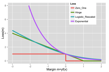
While exponential loss has nice theoretical and computational properties, it comes with a key drawback — lack of robustness.
Recall that the exponential loss is:
\[\ell_{\text{exp}}(y, f(x)) = \exp(-y f(x))\]
This function grows exponentially as the margin \(y f(x)\) becomes more negative. So:
- Misclassified examples (where \(y f(x) < 0\)) incur very high penalties.
- As a result, outliers or noisy labels can dominate the loss and heavily influence the model.
Practical Consequences
- AdaBoost (which minimizes exponential loss) tends to over-focus on misclassified points, even if they are noisy or mislabeled.
- This leads to degraded performance in datasets with:
- High Bayes error rate (i.e., intrinsic label uncertainty),
- Significant label noise.
In contrast, logistic loss (or log-loss), used in Logistic Regression, penalizes mistakes more gradually and is more robust in such settings.
Why Still Use Exponential Loss?
Despite these robustness concerns, exponential loss has some computational advantages:
- It leads to simpler update rules (as seen in AdaBoost),
- The math works out cleanly in boosting settings,
- It’s easy to implement and analyze.
So in summary:
Exponential loss is powerful and efficient but sensitive to outliers.
Logistic loss is more robust, especially when the data is noisy or inherently uncertain.
Wrapping up
In this post, we’ve unpacked how Forward Stagewise Additive Modeling (FSAM) builds models by greedily adding base learners — and how, when paired with the exponential loss, it naturally recovers the well-known AdaBoost algorithm.
Key takeaways:
- FSAM provides a clean, iterative framework for model building.
- The exponential loss leads to a simple and elegant form of weight updates.
- AdaBoost emerges as a special case of FSAM with exponential loss, emphasizing misclassified examples via weighted classification error and adaptive reweighting.
However, this formulation is limited to specific loss functions like the exponential loss.
What’s next?
In the upcoming post, we’ll generalize this framework to work with any differentiable loss function, leading to the powerful and flexible family of models known as Gradient Boosted Machines (GBMs).