Boosting and AdaBoost

Boosting is a powerful machine learning technique that focuses on reducing the error rate of high-bias estimators by combining many weak learners, typically trained sequentially. Unlike bagging, which trains classifiers in parallel to reduce variance, boosting focuses on improving performance by training classifiers sequentially on reweighted data. The core idea behind boosting is simple: rather than using a large and complex model that may overfit, we train a series of simpler models (typically decision trees) to improve accuracy gradually.

In contrast to bagging’s emphasis on parallel training of multiple models on different data subsets, boosting systematically reweights the training examples after each classifier is added, directing the model’s attention to examples that previous classifiers struggled with.

Key Intuition:

• A weak learner is a classifier that performs slightly better than random chance.
  • Example: A rule such as “If <keyword> then spam” or “From a friend” then “not spam”.
• Weak learners focus on different parts of the data, which may be misclassified by previous models.
• The final model is a weighted combination of these weak learners, with each learner contributing differently based on its performance.

We will explore a specific boosting algorithm: AdaBoost (Freund & Schapire, 1997), which is commonly used with decision trees as weak learners.

---

AdaBoost: Setting

For binary classification, where the target variable \(Y = \{-1, 1\}\), AdaBoost uses a base hypothesis space \(H = \{h : X \rightarrow \{-1, 1\}\}\). Common choices for weak learners include:

• Decision stumps: A tree with a single split.
• Decision trees with a few terminal nodes.
• Linear decision functions.

Weighted Training Set

Each weak learner in AdaBoost is trained on a weighted version of the training data. The training set \(D = \{(x_1, y_1), \dots, (x_n, y_n)\}\) has weights associated with each example: \(w_1, w_2, \dots, w_n\).

The weighted empirical risk is defined as:

\[\hat{R}_n^w(f) \overset{\text{def}}{=} \frac{1}{W} \sum_{i=1}^{n} w_i \cdot \ell(f(x_i), y_i)\]

where \(W = \sum_{i=1}^{n} w_i\), and \(\ell\) is a loss function (typically 0-1 loss in the case of classification).

Examples with larger weights have a more significant impact on the loss, guiding the model to focus on harder-to-classify examples.

AdaBoost: Sketch of the Algorithm

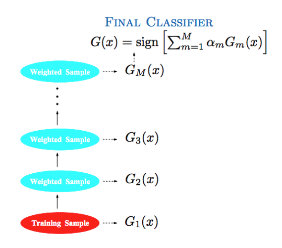
AdaBoost works by combining several weak learners to create a strong classifier.
Here’s the high-level process:

1. Start by assigning equal weights to all training examples:

\[w_1 = w_2 = \cdots = w_n = 1\]

1. For each boosting round \(m = 1, \dots, M\) (where \(M\) is the number of classifiers we want to train):

   • Train a base classifier \(G_m(x)\) on the current weighted training data.
   • Evaluate how well \(G_m(x)\) performs.
   • Increase the weights of examples that were misclassified, so the next classifier focuses more on those harder examples.

2. Aggregate the predictions from all classifiers, weighted by their accuracy:

\[G(x) = \text{sign}\left( \sum_{m=1}^{M} \alpha_m G_m(x) \right)\]

The key idea is: the more accurate a base learner, the higher its influence in the final prediction.

AdaBoost: How to Compute Classifier Weights

In AdaBoost, each base classifier \(G_m\) contributes to the final prediction with a weight \(\alpha_m\).
We want the following:

• \(\alpha_m\) should be non-negative.
• \(\alpha_m\) should be larger when \(G_m\) fits its weighted training data well.

The weighted 0-1 error of the base classifier \(G_m(x)\) is computed as:

\[\text{err}_m = \frac{1}{W} \sum_{i=1}^{n} w_i \, \mathbf{1}\left[ y_i \neq G_m(x_i) \right]\]

where:

• \(W = \sum_{i=1}^{n} w_i\) is the total sum of weights.
• \(\mathbf{1}[\cdot]\) is an indicator function, equal to 1 if the condition is true, and 0 otherwise.

Since the error is normalized by the total weight, we always have:

\[\text{err}_m \in [0, 1]\]

Once we know the error \(\text{err}_m\), we compute the weight of the classifier \(G_m\) as:

\[\alpha_m = \ln\left( \frac{1 - \text{err}_m}{\text{err}_m} \right)\]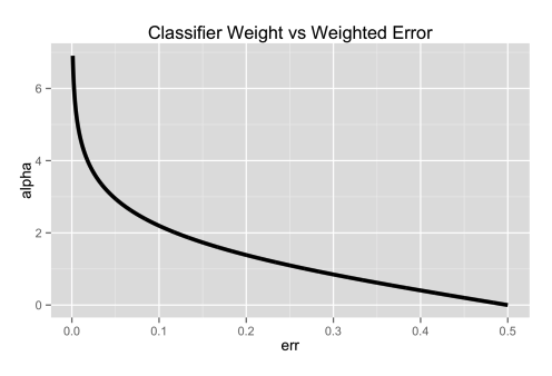

Interpretation:

• If \(\text{err}_m\) is small (good classifier), then \(\alpha_m\) is large.
• If \(\text{err}_m\) is large (poor classifier), then \(\alpha_m\) is small.

Thus, more accurate classifiers get higher voting power in the final decision.

AdaBoost: How Example Weights Are Updated

After training a base classifier, we update the weights of the examples to focus more on mistakes.

Suppose \(w_i\) is the weight of example \(x_i\) before training \(G_m\). After training:

• If \(G_m\) correctly classifies \(x_i\), keep \(w_i\) the same.
• If \(G_m\) misclassifies \(x_i\), increase \(w_i\):

\[w_i \leftarrow w_i \times e^{\alpha_m}\]

This adjustment ensures that:

• Hard examples (previously misclassified) get more weight and are more likely to be correctly classified by future classifiers.
• If \(G_m\) is a strong classifier (large \(\alpha_m\)), the weight update for misclassified examples is more significant.

Alternatively, you can think of it this way:

\[w_i \leftarrow w_i \times \left( \frac{1}{\text{err}_m} - 1 \right)\]

This reweighting step is what drives AdaBoost to sequentially correct the errors of the previous learners.

Intuition Behind AdaBoost: Analogy

To better internalize AdaBoost, imagine the process as training a team of tutors to help a student (the model) pass an exam (classification task):

• First Tutor: The first tutor teaches the entire syllabus equally. After the first test, they realize the student struggles with some topics (mistakes/misclassifications).

• Second Tutor: The second tutor focuses more heavily on the topics where the student made mistakes, spending extra time on them.

• Third Tutor: The third tutor notices there are still lingering problems on certain topics, so they focus even more narrowly on the hardest concepts.

• And so on…

Each tutor is not perfect, but by combining their focused efforts, the student gets a much more complete understanding — better than what any single tutor could achieve alone.

---

Simple Mathematical Example

Let’s walk through a tiny AdaBoost example to see everything in action.

Suppose we have 4 data points:

---

\(x_i\)	\(y_i\) (True Label)
1	+1
2	+1
3	-1
4	-1

---

Step 1: Initialization

All examples start with equal weight:

\[w_i = \frac{1}{4} = 0.25 \quad \text{for each } i\]

Step 2: First Classifier \(G_1(x)\)

Suppose \(G_1\) predicts:

---

\(x_i\)	\(G_1(x_i)\)
1	+1
2	-1 ❌
3	-1
4	-1

---

It misclassifies \(x_2\).

Compute weighted error:

\[\text{err}_1 = \frac{w_2}{\sum_{i=1}^{4} w_i} = \frac{0.25}{1} = 0.25\]

Classifier weight:

\[\alpha_1 = \ln\left( \frac{1 - 0.25}{0.25} \right) = \ln(3) \approx 1.0986\]

Step 3: Update Weights

Increase the weight for the misclassified example:

• For correctly classified points \(w_i\) stays the same.
• For misclassified points:

\[w_i \leftarrow w_i \times e^{\alpha_1}\]

Thus:

• \(w_2\) (misclassified) becomes:

\[w_2' = 0.25 \times e^{1.0986} \approx 0.25 \times 3 = 0.75\]

• \(w_1, w_3, w_4\) stay \(0.25\).

Normalization step (so weights sum to 1):

Total weight:

\[W' = 0.25 + 0.75 + 0.25 + 0.25 = 1.5\]

New normalized weights:

---

\(x_i\)	New Weight
1	\(\frac{0.25}{1.5} \approx 0.167\)
2	\(\frac{0.75}{1.5} = 0.5\)
3	\(\frac{0.25}{1.5} \approx 0.167\)
4	\(\frac{0.25}{1.5} \approx 0.167\)

---

Step 4: Second Classifier \(G_2(x)\)

Train next classifier \(G_2\) on the new weights.

Now, \(x_2\) has the highest weight (0.5), so the model focuses more on predicting \(x_2\) correctly!

(And the process repeats…)

Key Takeaways

• AdaBoost punishes mistakes by increasing weights of misclassified examples.
• Future classifiers focus on the harder examples.
• Classifier weight \(\alpha\) depends on how good the classifier is (lower error → higher weight).
• Final prediction is:

\[G(x) = \text{sign}\left( \alpha_1 G_1(x) + \alpha_2 G_2(x) + \cdots + \alpha_M G_M(x) \right)\]

Thus, even if each individual classifier is weak, together they become strong!

---

AdaBoost: Algorithm

Given a training set:

\[\mathcal{D} = \{(x_1, y_1), \ldots, (x_n, y_n)\}.\]

The AdaBoost procedure works as follows:

Steps:

1. Initialize observation weights:

   Set:

   \[w_i = 1, \quad \text{for all } i = 1, 2, \ldots, n.\]

2. For \(m = 1\) to \(M\) (number of base classifiers):

   • Train a base learner on the weighted training data, obtaining a classifier \(G_m(x)\).

   • Compute the weighted empirical 0-1 risk:

   \[\text{err}_m = \frac{1}{W} \sum_{i=1}^{n} w_i \, \mathbf{1}[y_i \neq G_m(x_i)],\]

   where:

   \[W = \sum_{i=1}^{n} w_i.\]

   • Compute classifier weight:

     Assign a weight to the classifier based on its error:

     \[\alpha_m = \ln\left( \frac{1 - \text{err}_m}{\text{err}_m} \right).\]

   • Update example weights:

     Update the training example weights to emphasize misclassified examples:

     \[w_i \leftarrow w_i \times \exp\left( \alpha_m \mathbf{1}[y_i \neq G_m(x_i)] \right).\]

3. Final classifier:

   After \(M\) rounds, return the final classifier:

   \[G(x) = \text{sign}\left( \sum_{m=1}^{M} \alpha_m G_m(x) \right).\]

To put it shortly:

• Start: Treat every sample equally.
• Learn: Focus the learner on samples that previous classifiers got wrong.
• Combine: Build a strong final classifier by combining the weighted votes of all the base classifiers.

Each \(\alpha_m\) ensures that better-performing classifiers get a stronger say in the final decision!

---

Weighted Error vs. Classifier’s True Error

In AdaBoost, the error \(\text{err}_m\) computed at each iteration is the weighted error based on the current distribution of sample weights, not the classifier’s true (unweighted) error rate over the data.

This distinction is important: a classifier might have a low overall misclassification rate but could still have a high weighted error if it misclassifies examples that currently have large weights (i.e., harder or previously misclassified points).

AdaBoost intentionally shifts focus toward difficult examples, so do not confuse the weighted empirical error used in boosting with the base learner’s standard classification error.

How is the Base Learner Optimized at Each Iteration?

At each iteration \(m\) of AdaBoost, the goal is to find the base classifier \(G_m(x)\) that minimizes the weighted empirical error:

\[\text{err}_m = \frac{1}{W} \sum_{i=1}^{n} w_i \, \mathbf{1}[y_i \neq G_m(x_i)].\]

Here’s the key idea:

• We don’t try to find a classifier that perfectly fits the original (unweighted) training data.
• Instead, we optimize for the current weighted dataset — meaning examples with larger weights influence the learning process more.
• The base learner is trained to focus on minimizing mistakes on the examples that have been harder to classify so far.

Typical Optimization Process:

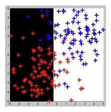
• If using decision stumps (one-level decision trees), the learner searches for the split that minimizes the weighted classification error.
• In general, the base model uses the sample weights as importance scores to guide its fitting.

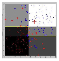
Thus, at each step, AdaBoost adapts the learning problem to focus on what the previous classifiers struggled with, gradually building a strong ensemble.

Does AdaBoost Overfit?

While boosting generally performs well, it’s natural to ask: Does AdaBoost overfit with many rounds?

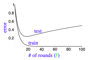
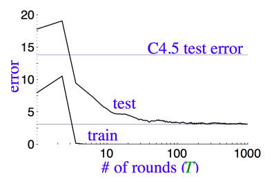
The learning curves for AdaBoost typically show that the test error continues to decrease even after the training error reaches zero, which indicates that AdaBoost is resistant to overfitting. This is one of the reasons why AdaBoost is so powerful: it can maintain good generalization even with many weak learners.

AdaBoost in Real-World Applications

A famous application of AdaBoost is face detection, as demonstrated in Viola & Jones (2001). In this case, AdaBoost uses pre-defined weak classifiers and employs a smart way of doing real-time inference, even on hardware from 2001. This demonstrates the efficiency and applicability of AdaBoost in practical scenarios.

Wrapping Up

Boosting is an ensemble technique aimed at reducing bias by combining multiple weak learners. The sequential nature of boosting means that each learner focuses on errors made by previous ones, ultimately improving the model’s performance. AdaBoost is a specific and highly effective boosting algorithm that can be used with decision trees as weak learners to achieve powerful classification results.

Next Steps:

In the next section, we’ll explore the objective function of AdaBoost in more detail, along with some generalizations to other loss functions and the popular Gradient Boosting algorithm.