BinomialBoost
In the previous post, we introduced the Gradient Boosting framework as functional gradient descent, where we minimize a loss function by iteratively adding base learners that approximate the negative gradient (pseudo-residuals) of the loss. We demonstrated this with the squared loss, where residuals had a direct and intuitive interpretation. In this post, we extend that idea to logistic loss, which is more appropriate for binary classification tasks. This special case is often referred to as BinomialBoost.
Logistic Loss and Pseudo-Residuals
For binary classification with labels \(Y = \{-1, 1\}\), the logistic loss is given by:
\[\ell(y, f(x)) = \log(1 + e^{-y f(x)})\]At each boosting iteration, we need to compute the pseudo-residuals, which are the negative gradients of the loss with respect to the model’s prediction. For the \(i\)-th training example:
\[\begin{aligned} r_i &= - \frac{\partial}{\partial f(x_i)} \ell(y_i, f(x_i)) \\ &= - \frac{\partial}{\partial f(x_i)} \log(1 + e^{-y_i f(x_i)}) \\ &= y_i \cdot \frac{e^{-y_i f(x_i)}}{1 + e^{-y_i f(x_i)}} \\ &= \frac{y_i}{1 + e^{y_i f(x_i)}} \end{aligned}\]These pseudo-residuals guide the model by indicating how each example’s prediction should be adjusted to reduce the classification loss.
Step Direction and Boosting Update
Once we compute the pseudo-residuals \(r_i\), the next base learner \(h_m \in \mathcal{H}\) is fit to match them in a least squares sense:
\[h_m = \arg\min_{h \in \mathcal{H}} \sum_{i=1}^n \left( \frac{y_i}{1 + e^{y_i f_{m-1}(x_i)}} - h(x_i) \right)^2\]The model is then updated as:
\[f_m(x) = f_{m-1}(x) + \nu h_m(x)\]where \(\nu \in (0, 1]\) is the learning rate or shrinkage parameter and \(f_{m-1}(x)\) is prediction after \(m−1\) rounds.
Gradient Tree Boosting
A particularly effective version of gradient boosting uses regression trees as base learners. The hypothesis space is:
\[\mathcal{H} = \{ \text{regression trees with } S \text{ terminal nodes} \}\]- \(S = 2\) corresponds to decision stumps, a very simple weak learner that makes a prediction based on a single feature threshold.
- Larger values of \(S\) allow more expressive trees, capable of capturing more complex interactions among features.
- Common choices for tree size: \(4 \leq S \leq 8\)
Gradient Tree Boosting combines the predictive power of decision trees with the optimization capabilities of functional gradient descent. Each tree fits the pseudo-residuals (i.e., the gradient of the loss), and the overall model evolves by sequentially adding these trees with appropriate scaling (via step size or shrinkage).
This approach is widely known as Gradient Tree Boosting and is implemented in various software packages:
- R:
gbm - scikit-learn:
GradientBoostingClassifier,GradientBoostingRegressor - XGBoost, LightGBM: state-of-the-art libraries for scalable, high-performance boosting
Visual Example;

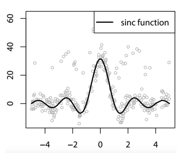
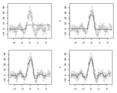
As a simple regression example, we can use an ensemble of decision stumps to fit a noisy version of the sinc function using squared loss. Even shallow learners (depth-1 trees) become powerful when combined via boosting. Here’s what the model looks like after different boosting rounds:

The shrinkage parameter \(\lambda = 1\) is used in this example to simplify learning, though smaller values are typically preferred in practice to prevent overfitting.
Conclusion
With all the pieces in place, we can summarize what’s needed to implement Gradient Boosting (also known as AnyBoost):
- A differentiable loss function: e.g., squared loss for regression, logistic loss for classification
- A base hypothesis space: e.g., regression trees of fixed depth
- A gradient descent procedure in function space
- Hyperparameters: step size \(\nu\), number of boosting rounds \(M\), tree size \(S\)
This general and flexible framework can adapt to a wide variety of tasks, making Gradient Boosting one of the most versatile and powerful tools in modern machine learning.