Decision Trees - Our First Non-Linear Classifier
So far, we’ve seen classifiers that try to separate data using straight lines or hyperplanes—like logistic regression and SVMs. But what happens when a linear boundary just doesn’t cut it?
Welcome to decision trees, our first inherently non-linear classifier. These models can slice the input space into complex shapes, enabling them to learn highly flexible rules for classification and regression.
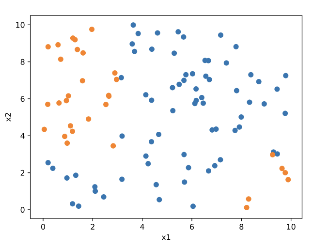
To understand the core idea, consider this question:

Can we classify these points using a linear classifier?
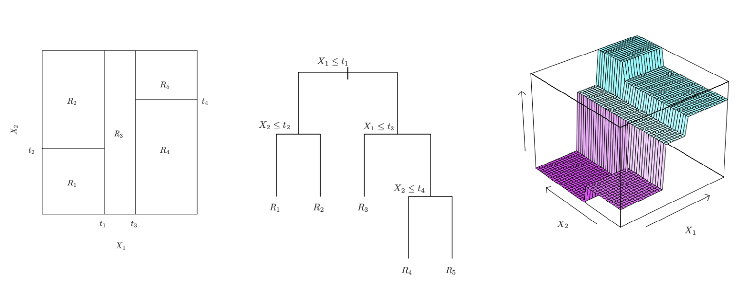
Sometimes the answer is no. In such cases, we can instead partition the input space into axis-aligned regions recursively. This is exactly what a decision tree does—it recursively divides the space based on feature thresholds, creating regions where simple predictions (like mean or majority label) are made.
Decision Trees: Setup
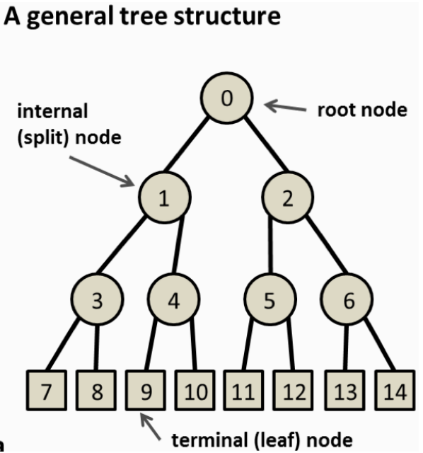
We’ll focus on binary decision trees, where each internal node splits the dataset into exactly two parts based on a single feature.

Key structure of a binary decision tree:
- Each node corresponds to a subset of the data.
- At every split, exactly one feature is used to divide the data.
- For continuous features, splits are typically of the form: \(x_i \leq t\) where \(t\) is a learned threshold.
- For categorical features, values can be partitioned into two disjoint groups (not covered in this post).
- Predictions are made only at the terminal nodes (also called leaves), where no further splitting occurs.
Constructing the Tree
Before we dive into the mechanics of decision trees, let’s understand the core objective:
We want to partition the input space into regions \(R_1, R_2, \ldots, R_J\) in a way that minimizes the prediction error in each region.
Formally, our aim is to find the regions \(R_1, \ldots, R_J\) that minimize the sum of squared errors within each region:
\[\sum_{j=1}^{J} \sum_{i \in R_j} (y_i - \hat{y}_{R_j})^2\]Here:
- \(y_i\) is the true target value,
- \(\hat{y}_{R_j}\) is the predicted value in region \(R_j\), typically the mean of \(y_i\)’s in that region.
Why this formulation?
This objective captures our desire to make accurate predictions within each region. By minimizing the sum of squared errors (SSE), we’re encouraging the model to place similar target values together. In other words, a good split should group data points that can be well-represented by a single value—their mean.
The mean minimizes the squared error within a region, making it the natural prediction for regression tasks. This also ensures that the tree focuses on reducing variance within each region, which is a core idea behind how decision trees generalize from data.
Intuition with a Simple Example:
Suppose you’re trying to predict someone’s salary based on their years of experience. If you create a region \(R_j\) that contains people with 2–4 years of experience and their salaries are: $45k, 48k, 46k, 47k$, then predicting the mean salary (≈ $46.5k) gives you the smallest total squared error.
But if you instead included someone with 10 years of experience and a salary of $80k in the same region, your prediction would shift higher—and the squared error for the 2–4 year group would increase significantly. So, to minimize overall error, we should split the region before including such an outlier. This is exactly what the tree tries to do—split the data where it significantly improves prediction accuracy.
In essence, the tree grows by trying to group together points that are similar in their target values—allowing for simple and accurate predictions within each region.
Problem: Intractability
While our goal is clear—split the data into regions that minimize prediction error—actually finding the optimal binary tree is computationally infeasible.
Why? Because the number of possible binary trees grows exponentially with the number of features and data points. At each node, we can choose any feature and any possible split value, and each choice affects all future splits. This creates an enormous search space.
Let’s go back to our salary prediction task. Suppose we have 100 employees with features like years of experience, education level, and job title. At the root node, we could split on:
- Experience: maybe at 5 years?
- Education: perhaps separate Bachelor’s from Master’s and PhDs?
- Job title: group certain roles together?
Each of these choices leads to different subsets of the data—then we repeat the process within each subset. Even for a small dataset, the number of ways to split and grow the tree quickly becomes astronomical.
Evaluating every possible combination of splits and tree structures to find the one that gives the absolute minimum prediction error would require checking all trees, which is practically impossible.
Solution: Greedy Construction
Instead of searching the entire tree space, we use a greedy algorithm:
- Start at the root node with the full dataset.
- Evaluate all possible splits and choose the one that minimizes the error locally.
- Split the data accordingly.
- Repeat the process recursively until a stopping condition is met, such as:
- Reaching a maximum tree depth,
- A minimum number of data points in a node,
- Or achieving a minimal decrease in error.
💡 We only split regions that have already been defined by earlier (non-terminal) splits. So the tree structure builds hierarchically, and each decision is context-dependent.
Prediction in Terminal Nodes
Once the tree is built, how do we make predictions?
For regression, the predicted value at a terminal node \(R_m\) is just the average of the targets in that region:
\[\hat{y}_{R_m} = \text{mean}(y_i \mid x_i \in R_m)\]
Greedy Nature and Its Implications
This greedy approach makes locally optimal decisions at each step without considering their long-term impact. As a result:
- It is efficient and straightforward to implement.
- However, it may not lead to the globally optimal tree, since better overall structures might require different early splits.
Example:
Suppose we’re predicting salary and at the root node, we greedily choose to split on education level, since it gives the best reduction in squared error at that moment.
But later, we realize that years of experience would have provided a much cleaner separation if it had been split first. Unfortunately, the tree can’t go back and revise that decision.
That’s the key limitation of greedy methods:
They make the best decision in the moment—but not necessarily the best decision overall.
How do we find the best split point?
When building decision trees, we need to decide where to split the data at each node. Here’s how it’s typically done:
-
Step 1: Iterate over all features.
For each feature, we try to find the best possible threshold that minimizes the loss (e.g., squared error). -
Step 2: Handle continuous features efficiently.
While there are infinitely many possible split points for continuous features, we don’t need to try them all.
Key Insight:
If we sort the values of a feature \(x_j\), say:
\[x_{j(1)}, x_{j(2)}, \ldots, x_{j(n)}\]then we only need to consider splits between adjacent values. Why?
Because any split point within the interval \((x_{j(r)}, x_{j(r+1)})\) will result in the same data partition, and hence the same loss.
Common Strategy:
We pick the midpoint between adjacent sorted values as the candidate split:
\[s_j \in \left\{ \frac{1}{2} \left(x_{j(r)} + x_{j(r+1)}\right) \,\middle|\, r = 1, \ldots, n - 1 \right\}\]So instead of testing infinitely many thresholds, we reduce the search to just \(n - 1\) candidate splits for each feature—making the process tractable and efficient.
Decision Trees and Overfitting
What happens if we keep splitting the data?
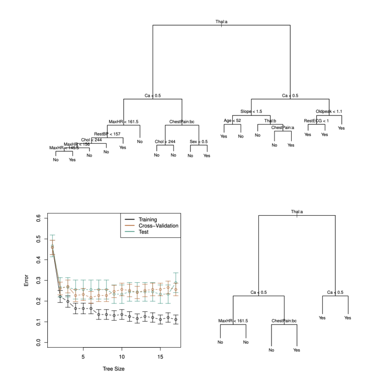
Eventually, the tree can grow so deep that every leaf contains just one data point. This means the model has memorized the training data—resulting in zero training error, but likely poor generalization to unseen data.
In other words: overfitting.
To prevent this, we need to regularize the tree by controlling its complexity. Common strategies include:
- Limit the depth of the tree
- Limit the total number of nodes
- Restrict the number of terminal (leaf) nodes
- Set a minimum number of samples required to split a node or to be in a leaf
Another strategy is pruning, which is used in the famous CART algorithm (Breiman et al., 1984):
- Grow a large tree: Allow the tree to grow deep, often until each leaf contains just a few data points (e.g., ≤ 5).
- Prune it back: Starting from this large tree, recursively remove subtrees if doing so improves performance on a validation set.
This two-phase approach ensures the model starts expressive but is ultimately simplified to avoid overfitting.

Wrapping Up:
-
Decision Trees are a powerful method that recursively splits the data to minimize prediction error, enabling flexible models for both regression and classification tasks.
-
The Greedy Approach is used to make locally optimal decisions at each split, though it may not always lead to the globally best tree.
-
Overfitting is a concern when the tree becomes too complex, which can be mitigated by using regularization techniques like limiting depth and pruning.
-
Pruning simplifies the tree after it has been grown, helping to avoid overfitting and improve generalization.
Now that we’ve explored decision trees in a regression context, let’s shift gears and dive into how they work for classification. Specifically, we’ll focus on understanding what constitutes a good split in classification and how to define the misclassification error in a node. Let’s dive into these topics in the next post.
See you!