Decision Trees for Classification
In the last post, we explored how decision trees can grow deep and complex—leading to overfitting—and how strategies like limiting tree depth or pruning can help us build simpler, more generalizable models.
In this post, we turn our focus to classification trees, where our goal isn’t just fitting the data—it’s finding splits that create pure, confident predictions in each region.
We’ll look at what makes a split “good,” explore different impurity measures, and understand how decision trees use these ideas to grow meaningfully.
What Makes a Good Split for Classification?
In classification tasks, a decision tree predicts the majority class in each region. So, a good split is one that increases the purity of the resulting nodes—that is, each node contains mostly (or only) examples from a single class.
Let’s walk through a concrete example. Suppose we’re trying to classify data points into positive (+) and negative (−) classes. We consider two possible ways to split the data:
Split Option 1
- \[R_1: 8+,\ 2−\]
- \[R_2: 2+,\ 8−\]
Here, each region contains a clear majority: 8 out of 10 are of the same class. Not bad!
Split Option 2
- \[R_1: 6+,\ 4−\]
- \[R_2: 4+,\ 6−\]
This is more mixed—each region has a 60-40 class split, making it less pure than Split 1.
Now, let’s consider a better version of Split 2:
Split Option 3 (Refined)
- \[R_1: 6+,\ 4−\]
- \[R_2: 0+,\ 10−\]
Now things look different! Region \(R_2\) contains only negatives, making it a perfectly pure node. Even though \(R_1\) isn’t completely pure, this split overall is more desirable than the others.
This example shows that a good split isn’t just about balance—it’s about maximizing purity, ideally pushing each node toward containing only one class.
Misclassification Error in a Node
Once we split the data, how do we measure how well a node performs in classification?
Suppose we’re working with multiclass classification, where the possible labels are:
\[Y = \{1, 2, \ldots, K\}\]Let’s focus on a particular node \(m\) (i.e., a region \(R_m\) of the input space) that contains \(N_m\) data points.
For each class \(k \in \{1, \ldots, K\}\), we compute the proportion of points in node \(m\) that belong to class \(k\):
\[\hat{p}_{mk} = \frac{1}{N_m} \sum_{i: x_i \in R_m} \mathbb{1}[y_i = k]\]This gives us the empirical class distribution within the node.
To make a prediction, we choose the majority class in that node:
\[k(m) = \arg\max_k \hat{p}_{mk}\]This means the class with the highest proportion becomes the predicted label for all points in that region.
Node Impurity Measures
In classification, our goal is to make each region (or node) as pure as possible—i.e., containing data points from mostly one class.
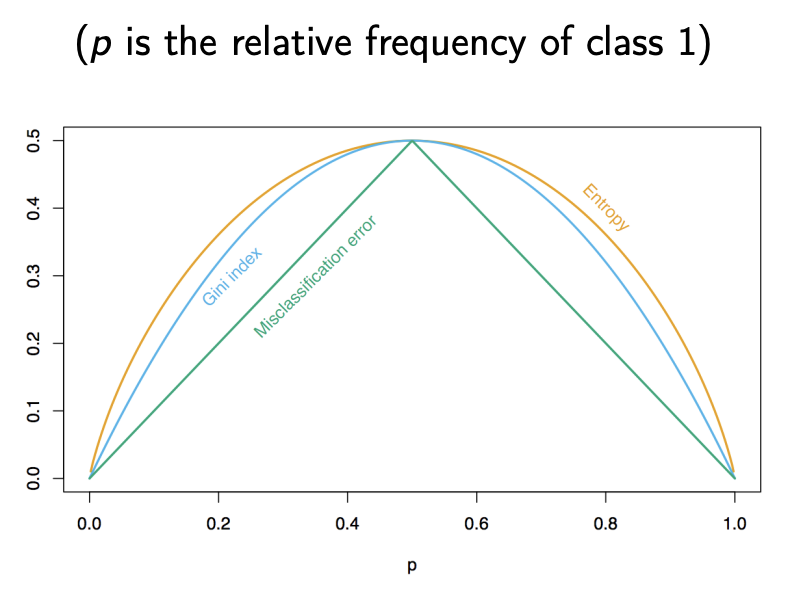
To quantify how impure a node is, we use impurity measures. Let’s explore the three most common ones:
1. Misclassification Error
This measures the fraction of points not belonging to the majority class in a node:
\[\text{Misclassification Error} = 1 - \hat{p}_{mk(m)}\]Here, \(\hat{p}_{mk(m)}\) is the proportion of the majority class in node \(m\).
- If a node has 90% of points from class A and 10% from class B, misclassification error = \(1 - 0.9 = 0.1\)
- It’s simple, but not very sensitive to class distribution beyond the majority vote.
2. Gini Index
The Gini index gives us a better sense of how mixed a node is:
\[\text{Gini}(m) = \sum_{k=1}^K \hat{p}_{mk}(1 - \hat{p}_{mk})\]This value is 0 when the node is perfectly pure (i.e., all points belong to one class) and maximum when all classes are equally likely.
- For example, if a node has:
- 50% class A, 50% class B → Gini = \(0.5\)
- 90% class A, 10% class B → Gini = \(0.18\)
- 100% class A → Gini = \(0\) (pure)
The Gini index is widely used in practice because it’s differentiable and more sensitive to class proportions than misclassification error.
3. Entropy (a.k.a. Information Gain)
Entropy comes from information theory and captures the amount of uncertainty or disorder in the class distribution:
\[\text{Entropy}(m) = - \sum_{k=1}^K \hat{p}_{mk} \log \hat{p}_{mk}\]Like Gini, it’s 0 for a pure node and higher for more mixed distributions.
- If a node has:
- 50% class A, 50% class B → Entropy = \(0.693\)
- 90% class A, 10% class B → Entropy ≈ \(0.325\)
- 100% class A → Entropy = \(0\)
Entropy grows slower than Gini but still encourages purity. It’s used in algorithms like ID3 and C4.5.
Summary: When Are Nodes “Pure”?
All three measures hit zero when the node contains data from only one class. But Gini and Entropy give a smoother, more nuanced view of how mixed the classes are—helpful for greedy splitting.
| Class Distribution | Misclassification | Gini | Entropy |
|---|---|---|---|
| 100% A | 0 | 0 | 0 |
| 90% A / 10% B | 0.1 | 0.18 | 0.325 |
| 50% A / 50% B | 0.5 | 0.5 | 0.693 |
So, when deciding where to split, we prefer splits that lead to lower impurity in the resulting nodes.

Analogy: Sorting Colored Balls into Boxes
Imagine you’re sorting colored balls into boxes. Each ball represents a data point, and the color represents its class label.
- A perfectly sorted box has balls of only one color—this is a pure node.
- A box with a mix of colors is impure—you’re less certain what color a randomly chosen ball will be.
Now think of impurity measures as ways to score each box. To ground these interpretations with some math, let’s calculate each impurity measure using a simple example.
Suppose we’re at a node where the class distribution is:
- 8 red balls (Class A)
- 2 blue balls (Class B)
This gives us the class probabilities:
- \[\hat{p}_A = \frac{8}{10} = 0.8\]
- \[\hat{p}_B = \frac{2}{10} = 0.2\]
Let’s compute each impurity measure and interpret what it tells us:
Misclassification Error: “What’s the chance I assign the wrong class if I always predict the majority class?”
- The majority class is red (Class A), so we’ll predict red for all inputs.
- The only mistakes occur when the true class is blue.
- So, the misclassification error is:
Gini Index: “If I randomly pick two balls (with replacement), what’s the chance they belong to different classes?”
- Formula:
- For our example:
- Interpretation: There’s a 32% chance of getting different classes when picking two random samples. The more balanced the classes, the higher the Gini.
Entropy: “How surprised am I when I pick a ball and see its class?”
- Formula:
- For our example:
- Approximating:
- Interpretation: Entropy is a measure of uncertainty. A pure node has zero entropy. Here, there’s moderate uncertainty because the node isn’t completely pure.
This example shows how the impurity measures behave when the node is somewhat pure but not perfectly. Gini and entropy are more sensitive to changes in class proportions than misclassification error, which is why they’re often preferred during tree building.
Quantifying the Impurity of a Split
Once we’ve chosen an impurity measure (like Gini, Entropy, or Misclassification Error), how do we decide if a split is good?
When a split divides a node into two regions—left (\(R_L\)) and right (\(R_R\))—we compute the weighted average impurity of the child nodes:
\[\text{Impurity}_{\text{split}} = \frac{N_L \cdot Q(R_L) + N_R \cdot Q(R_R)}{N_L + N_R}\]Where:
- \(N_L, N_R\) are the number of samples in the left and right nodes.
- \(Q(R)\) is the impurity of region \(R\), measured using Gini, Entropy, or Misclassification Error.
We want to minimize this weighted impurity. A good split is one that sends the data into two groups that are as pure as possible.
Example:
Suppose we split a node of 10 samples into:
- Left node (\(R_L\)): 6 samples, Gini impurity = 0.1
- Right node (\(R_R\)): 4 samples, Gini impurity = 0.3
Then the weighted impurity is:
\[\frac{6 \cdot 0.1 + 4 \cdot 0.3}{10} = \frac{0.6 + 1.2}{10} = 0.18\]We’d compare this value with the weighted impurity of other candidate splits and choose the split with the lowest value.
This process is repeated greedily at each step of the tree-building process.
Interpretability of Decision Trees

One of the biggest advantages of decision trees is their interpretability.
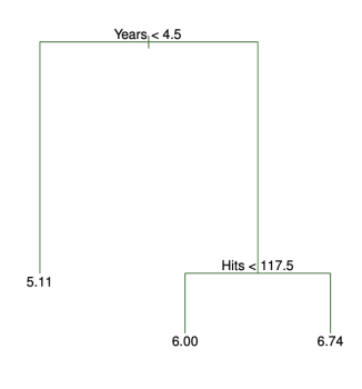
Each internal node represents a question about a feature, and each leaf node gives a prediction. You can follow a path from the root to a leaf to understand exactly how a prediction was made.
This makes decision trees particularly useful when model transparency is important—such as in healthcare or finance.
Even people without a technical background can often understand a small decision tree just by reading it. However, as trees grow deeper and wider, they can become harder to interpret, especially if overfit to the training data.
Discussion: Trees vs. Linear Models

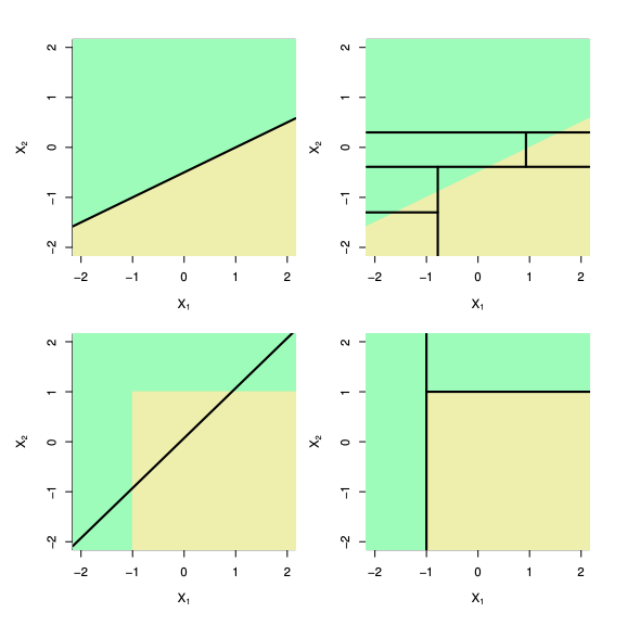
Unlike models like logistic regression or SVMs, decision trees don’t rely on geometric concepts such as distances, angles, or dot products. Instead, they work by recursively splitting the input space.
Decision trees are:
- Non-linear: They can carve out complex, axis-aligned regions in the input space.
- Non-metric: No need to define or compute distances between points.
- Non-parametric: They don’t assume a fixed form for the underlying function—tree complexity grows with data.
But there are tradeoffs:
- Trees may struggle with problems that have linear decision boundaries, which linear models handle easily.
- They are high-variance models—small changes in the training data can lead to very different trees.
- Without constraints (like pruning or depth limits), they are prone to overfitting, especially on noisy data.
Recap & Conclusion
-
Trees partition the input space into regions, unlike linear models that rely on fixed decision boundaries.
-
Split the data to minimize the sum of squared errors in each region.
-
Building the best tree is computationally infeasible. We use a greedy algorithm to build the tree step-by-step.
-
Fully grown trees overfit. We prevent this by limiting depth, size, or pruning based on validation performance.
-
For classfication, a good split increases class purity in the nodes. We explored this with intuitive +/− examples.
-
Impurity Measures: Misclassification Error, Gini Index and Entropy
-
We pick splits that reduce weighted impurity the most.
-
Small trees are easy to understand; large ones can become complex.
-
Trees are non-linear, non-parametric, and don’t need distance—but they may overfit or struggle with linear patterns.
This sets the stage for the next step: ensembles like Random Forests and Boosted Trees.
Stay tuned!