CS Fundamentals Refresher - Sorting, Hash Tables, and Matrix Multiplication
Hello all. This one is a refresher, not a deep dive. Three questions come up in almost every CS screening conversation, and they are the kind of thing that is easy to half-answer after a few years away from a textbook: how the standard sorts work and what they cost, why a hash table lookup is \(O(1)\) and what that data structure actually looks like in memory, and how much a matrix multiply costs when the matrices are not square. I could sketch each of these but not defend them, which is the worst place to be. So this post rebuilds all three from the ground up, at the level of detail where you can derive the answer instead of remembering it.
The angle throughout is the same one I use for GPU work: count the operations, then count the bytes, and notice that the second number usually explains the first. Every complexity in here comes from a recurrence or a counting argument you can redo on a whiteboard, and the library facts (what Python’s sort actually is, how a CPython dict is laid out) are pulled from the source with a date stamp.
The plan:
- The numbers that drive everything: the vocabulary, a table of what \(n \log n\) means at scale, and the one recurrence pattern behind every divide-and-conquer bound
- Sorting: the landscape, why \(n \log n\) is the floor, merge sort and quicksort from their recurrences, what real libraries run, and how counting and radix sort get under the floor
- Hash tables: the key to bucket contract, the two memory layouts, why lookups are \(O(1)\) and when they are not, and one concrete layout (the CPython dict)
- Matrix multiplication: the \(mnk\) count, irregular shapes, why the order of a chain of products matters, and how far below cubic anyone has gotten
- Test yourself: a question bank over everything above
Code is Python throughout, kept short enough to hold in your head. Let’s get started.
The Numbers That Drive Everything
The vocabulary
Five words carry most of the weight in any complexity conversation, and interviewers listen for whether you use them precisely.
| Term | What it means | Where it shows up below |
|---|---|---|
| Worst case | The maximum cost over all inputs of size \(n\) | Quicksort’s \(O(n^2)\), a hash table with every key in one bucket |
| Expected (average) case | The mean cost over the randomness, either in the input distribution or in the algorithm’s own coin flips | Randomized quicksort, hash table lookups |
| Amortized | The average cost per operation over a long sequence, even though a single operation can be expensive | Hash table resizing |
| In place | Uses \(O(1)\) or \(O(\log n)\) extra memory beyond the input | Quicksort yes, merge sort no |
| Stable | Equal keys keep their input order | Merge sort yes, quicksort no |
The distinction that matters most: an expected bound is a statement about randomness, an amortized bound is a statement about sequences, and neither is a worst-case guarantee for one operation. A hash table insert is \(O(1)\) expected and amortized, and \(O(n)\) in the worst case for a single call. All three statements are true at once, and being able to say which one you mean is the whole game.
What n log n means at scale
Asymptotic notation hides the constants, so it pays to have the actual magnitudes in your head. Using \(\log_2 10^3 \approx 10\), \(\log_2 10^6 \approx 20\), and \(\log_2 10^9 \approx 30\):
| \(n\) | \(\log_2 n\) | \(n \log_2 n\) | \(n^2\) | \(n^3\) |
|---|---|---|---|---|
| \(10^3\) | \(\approx 10\) | \(\approx 10^4\) | \(10^6\) | \(10^9\) |
| \(10^6\) | \(\approx 20\) | \(\approx 2 \times 10^7\) | \(10^{12}\) | \(10^{18}\) |
| \(10^9\) | \(\approx 30\) | \(\approx 3 \times 10^{10}\) | \(10^{18}\) | \(10^{27}\) |
Two things to take from the table. First, \(n \log n\) is barely worse than linear: at a billion elements the log factor is 30. That is why sorting is treated as “essentially free” in so many algorithms. Second, the gap between \(n \log n\) and \(n^2\) is enormous at any realistic \(n\), which is why the quicksort worst case is not an academic footnote. A million-element sort going quadratic is the difference between twenty million operations and a trillion.
The recurrence pattern behind everything
Every divide-and-conquer bound in this post comes out of one template. An algorithm that does \(f(n)\) non-recursive work and then makes \(r\) recursive calls on inputs of size \(n/c\) satisfies
\[T(n) = r \, T(n/c) + f(n)\]The clean way to solve it is the recursion tree, which is how Erickson’s Algorithms (chapter 1, section on recursion trees) presents it: draw the root with value \(f(n)\), give it \(r\) children each with value \(f(n/c)\), and keep going. The tree has \(\log_c n\) levels, and the number of leaves is \(r^{\log_c n} = n^{\log_c r}\). The total is the sum over levels, and that sum has exactly three shapes:
| Case | Condition | Total | Example |
|---|---|---|---|
| Root dominates | Level sums shrink geometrically going down | \(O(f(n))\) | \(T(n) = T(n/2) + n\) gives \(O(n)\) |
| All levels equal | Every level sums to about \(f(n)\) | \(O(f(n) \log n)\) | \(T(n) = 2T(n/2) + n\) gives \(O(n \log n)\) |
| Leaves dominate | Level sums grow geometrically going down | \(O(n^{\log_c r})\) | \(T(n) = 8T(n/2) + n^2\) gives \(O(n^3)\) |
Merge sort is the middle row. Strassen’s matrix multiply, at the end of the post, is the bottom row with \(r = 7\). And the quicksort worst case is not on the table at all, because when the split is \(n - 1\) against \(0\) the tree is a chain of depth \(n\) rather than a tree of depth \(\log n\), and the level sums \(n, n-1, n-2, \ldots\) add up to \(O(n^2)\).
References
- Jeff Erickson, Algorithms, chapter 1: Recursion (the recursion tree method and its three cases)
- Jeff Erickson, Algorithms, book index
Sorting
The landscape
Every sort below either compares pairs of elements or does not, and that one distinction decides whether it can beat \(n \log n\). Costs are in comparisons for the comparison sorts and in array accesses for the others. “Extra space” excludes the input array.
| Algorithm | How it works, in one line | Best | Average | Worst | Extra space | Stable | Comparison sort |
|---|---|---|---|---|---|---|---|
| Bubble sort | Repeatedly swap adjacent out-of-order pairs; each pass floats the max to the end | \(n\) | \(n^2\) | \(n^2\) | \(O(1)\) | Yes | Yes |
| Selection sort | Find the minimum of the unsorted suffix, swap it to the front, repeat | \(n^2\) | \(n^2\) | \(n^2\) | \(O(1)\) | No | Yes |
| Insertion sort | Take the next element, shift it left until it sits in order | \(n\) | \(n^2\) | \(n^2\) | \(O(1)\) | Yes | Yes |
| Merge sort | Split in half, sort each half, merge | \(n \log n\) | \(n \log n\) | \(n \log n\) | \(O(n)\) | Yes | Yes |
| Quicksort | Pick a pivot, partition around it, sort each side | \(n \log n\) | \(n \log n\) | \(n^2\) | \(O(\log n)\) stack | No | Yes |
| Heapsort | Build a max-heap, repeatedly pop the max to the end | \(n \log n\) | \(n \log n\) | \(n \log n\) | \(O(1)\) | No | Yes |
| Timsort | Find natural runs, extend short ones with insertion sort, merge runs | \(n\) | \(n \log n\) | \(n \log n\) | \(O(n)\) | Yes | Yes |
| Introsort | Quicksort, but switch to heapsort if recursion gets too deep | \(n \log n\) | \(n \log n\) | \(n \log n\) | \(O(\log n)\) | No | Yes |
| Counting sort | Count occurrences of each key in \([0, k)\), prefix-sum, place | \(n + k\) | \(n + k\) | \(n + k\) | \(O(n + k)\) | Yes | No |
| Radix sort (LSD) | Counting sort on each of \(d\) digits, least significant first | \(d(n + b)\) | \(d(n + b)\) | \(d(n + b)\) | \(O(n + b)\) | Yes | No |
A few of the entries deserve their sources. Selection sort uses about \(n^2/2\) compares and exactly \(n\) exchanges; insertion sort on random distinct keys uses about \(n^2/4\) compares and \(n^2/4\) exchanges on average, and its compare count is bounded by the number of inversions plus \(n\), which is why it is linear on nearly sorted input (Sedgewick and Wayne, Elementary Sorts). Heapsort uses fewer than \(2n \log_2 n\) compares and exchanges (Sedgewick and Wayne, Priority Queues). Bubble sort’s bound is just \(n - 1\) passes of up to \(n - 1\) compares each, and it is in the table only because interviewers still mention it; nobody ships it. The Timsort and introsort rows are what Python and C++ actually run, covered below.
Two rows are worth pausing on for the interview. Insertion sort is the answer to “which \(O(n^2)\) sort would you ever use?” because it is linear on nearly sorted data and has the lowest constant of the simple sorts, which is exactly why merge-based library sorts fall back to it for short runs. And heapsort is the answer to “\(n \log n\) worst case, in place, which one?” even though it is rarely the fastest, because it is the only row with both properties.
Why n log n is the floor
The claim to be able to reproduce: no algorithm that learns about its input only by comparing pairs of elements can sort in fewer than \(\Omega(n \log n)\) comparisons in the worst case.
The argument, following Erickson’s Lower Bounds notes (section 12.5), models the algorithm as a decision tree. Each internal node is a comparison “is \(x_i < x_j\)?”, each edge is an answer, and each leaf is the permutation the algorithm outputs. A correct sorter must be able to output every one of the \(n!\) permutations, so the tree has at least \(n!\) leaves. A binary tree with \(L\) leaves has depth at least \(\log_2 L\), and the depth of the tree is the number of comparisons on the worst path. So the worst case is at least \(\log_2(n!)\) comparisons. Stirling’s approximation gives \(n! > (n/e)^n\), hence
\[\log_2(n!) > n \log_2 n - n \log_2 e = \Omega(n \log n)\]That is the whole proof, and it is worth noticing what it does and does not say. It applies to any algorithm whose branching is driven only by comparisons: bubble, selection, insertion, merge, quick, heap, all of them. It does not apply to counting sort or radix sort, because they branch on the key’s value rather than on a comparison, and that is exactly how they beat the bound. Sedgewick states the same result as a compare count: no compare-based sort can guarantee fewer than \(\log_2(n!) \sim n \log_2 n\) compares (Mergesort).
Merge sort, from the recurrence
Merge sort is the cleanest instance of divide and conquer: split the array in half, sort each half recursively, then merge the two sorted halves into one. All the work is in the merge, and the merge is a single pass with two read pointers.
def merge_sort(a):
    if len(a) <= 1:
        return a
    mid = len(a) // 2
    left, right = merge_sort(a[:mid]), merge_sort(a[mid:])
    return merge(left, right)

def merge(left, right):
    out, i, j = [], 0, 0
    while i < len(left) and j < len(right):
        if left[i] <= right[j]:          # <= keeps equal keys in input order: stable
            out.append(left[i]); i += 1
        else:
            out.append(right[j]); j += 1
    out.extend(left[i:]); out.extend(right[j:])
    return out
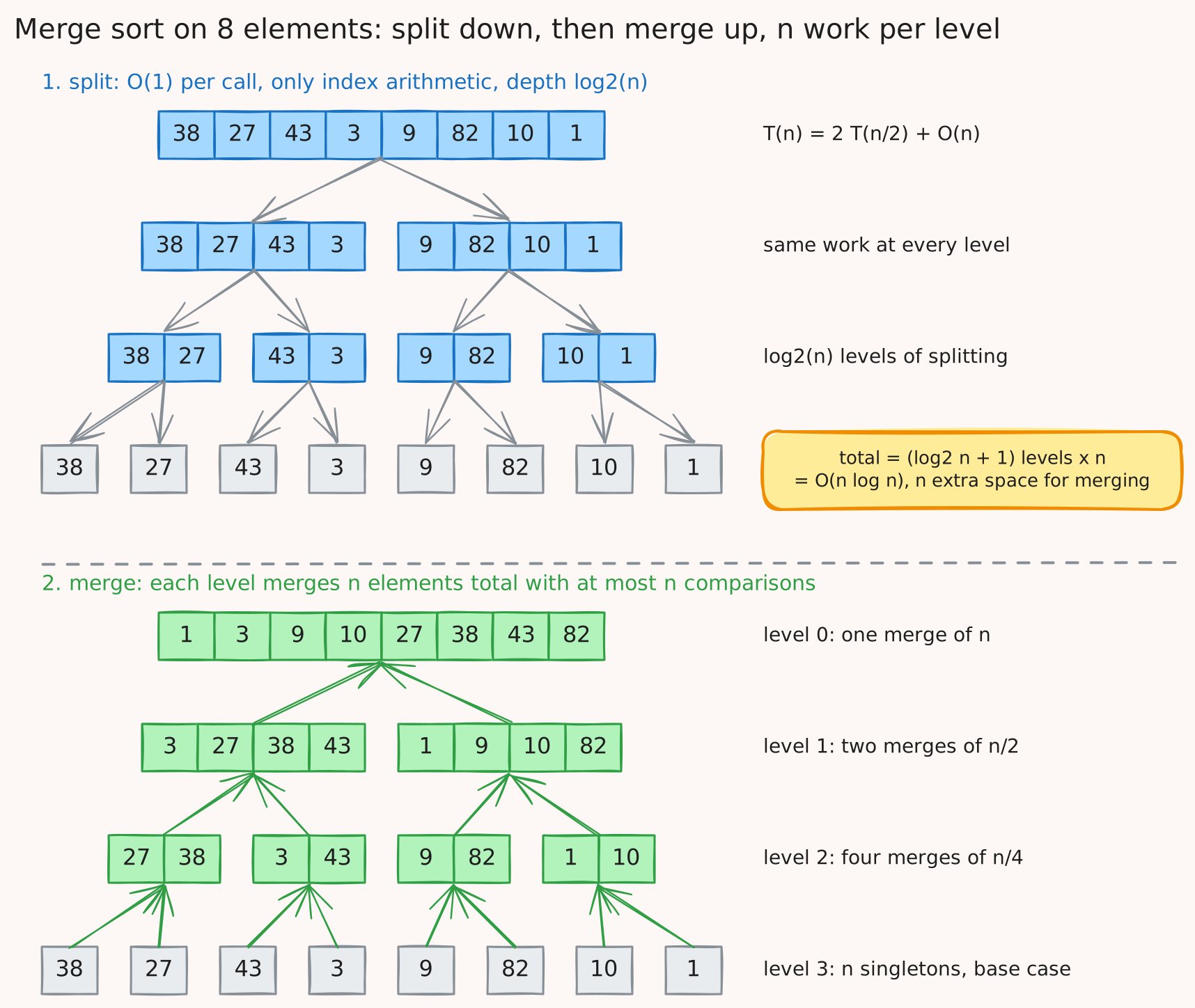
The merge does at most one comparison per element it emits, so merging two halves of total length \(n\) costs \(O(n)\). That gives the recurrence Erickson writes as \(T(n) = T(\lceil n/2 \rceil) + T(\lfloor n/2 \rfloor) + O(n)\), which after dropping the floors and ceilings is
\[T(n) = 2 \, T(n/2) + O(n) \quad \Longrightarrow \quad T(n) = O(n \log n)\]This is the “all levels equal” case from the recursion tree: the root merges \(n\) elements, its two children merge \(n/2\) each for a total of \(n\), the four grandchildren merge \(n/4\) each for a total of \(n\), and so on for \(\log_2 n\) levels (Erickson, chapter 1).
The properties worth being able to state without hesitation:
- Worst case equals best case. The split is always exactly in half regardless of the data, so the bound is \(\Theta(n \log n)\) for every input. Sedgewick’s precise count: between \(\tfrac{1}{2} n \log_2 n\) and \(n \log_2 n\) compares, and at most \(6 n \log_2 n\) array accesses (Mergesort).
- Stable, as long as the merge takes from the left half on ties, which is what the
<=in the code does. - Not in place. The merge needs a scratch buffer of size \(n\) (or \(n/2\) with care). This is the one real cost relative to quicksort, and the reason quicksort tends to win on arrays in memory.
- Sequential access. Both the split and the merge read and write contiguously, which is why merge sort is the natural choice for linked lists and for external sorting, where the data lives on disk and you merge runs that fit in memory.
The recursive version above allocates new lists at every level, which is fine for understanding and terrible for performance. A production merge sort works on index ranges in a single scratch buffer, and the bottom-up variant skips the recursion entirely by merging runs of length 1, then 2, then 4, and so on.
Quicksort, from the recurrence
Quicksort inverts merge sort: do the hard work before recursing, so that there is nothing to do after. Choose a pivot, partition the array so everything smaller than the pivot is on its left and everything larger on its right, and then recursively sort the two sides. The pivot is already in its final position and never moves again. Erickson credits the algorithm to Tony Hoare (chapter 1, section 1.5).
The partition is the part people get asked to write on a whiteboard. The version below is the Lomuto scheme: one pointer \(j\) scans left to right, another pointer \(i\) marks the end of the “less than or equal to pivot” region, and every time the scan finds a small element it swaps it into that region.
def quicksort(a, lo=0, hi=None):
    if hi is None:
        hi = len(a) - 1
    if lo < hi:
        p = partition(a, lo, hi)
        quicksort(a, lo, p - 1)
        quicksort(a, p + 1, hi)

def partition(a, lo, hi):
    pivot = a[hi]                    # last element as pivot (bad choice on sorted input, see below)
    i = lo - 1                       # a[lo..i] <= pivot
    for j in range(lo, hi):          # a[i+1..j-1] > pivot
        if a[j] <= pivot:
            i += 1
            a[i], a[j] = a[j], a[i]
    a[i + 1], a[hi] = a[hi], a[i + 1]
    return i + 1                     # pivot's final index
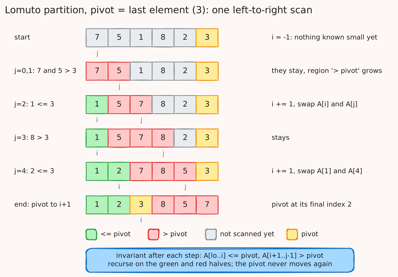
Hoare’s original partition scans from both ends toward the middle and swaps pairs that are on the wrong side. Its invariants are fiddlier to state, which is why Lomuto is what most people write under time pressure.
Partition is a single pass, so it costs \(O(n)\). The recurrence depends on where the pivot lands. If the pivot ends up at rank \(r\), Erickson writes
\[T(n) = T(r - 1) + T(n - r) + O(n)\]and the whole analysis is a case split on \(r\) (Erickson, chapter 1):
| Pivot lands at | Recurrence | Solution | When it happens |
|---|---|---|---|
| The median | \(T(n) = 2T(n/2) + O(n)\) | \(O(n \log n)\) | You paid for a linear-time median (never done in practice) |
| Anywhere in the middle tenth to ninth tenth | Two subproblems both a constant fraction smaller | \(O(n \log n)\) | Random pivot, most of the time |
| An end, \(r = 1\) or \(r = n\) | \(T(n) = T(n - 1) + O(n)\) | \(O(n^2)\) | First or last element as pivot on already sorted input |
| Second from an end, \(r = 2\) or \(r = n - 1\) | \(T(n) = T(n - 2) + O(n)\) | Still \(O(n^2)\) | Median-of-three on adversarial input |
The third row is the classic trap and worth saying out loud in an interview: with the first or last element as pivot, an already sorted array is the worst case, not the best. Every partition peels off one element, the recursion is \(n\) deep, and the total is \(n + (n-1) + \cdots = O(n^2)\). Median-of-three (take the median of the first, middle, and last elements) fixes sorted input and is a real improvement in practice, but Erickson’s point is that it does not fix the worst case; an adversary can still force \(r = 2\) every time.
The fix that actually works is randomization. If the pivot index is chosen uniformly at random, quicksort runs in \(O(n \log n)\) time with high probability for every possible input, because the randomness now belongs to the algorithm rather than to whoever chose the input (Erickson, chapter 1). The expected constant is known precisely: about \(2n \ln n\) compares and one sixth as many exchanges on distinct keys (Sedgewick and Wayne, Quicksort). Since \(2 \ln n = 2 \ln 2 \cdot \log_2 n \approx 1.39 \log_2 n\), that is about 39 percent more compares than merge sort’s upper bound, and quicksort still wins in practice. The reasons are the bytes, not the compares: it works in place with no scratch buffer, the partition scan is a sequential sweep that the cache and prefetcher love, and it moves far less data than merge sort, which copies every element at every level.
Three practical notes that round out the answer:
- Stack depth. Naive recursion can go \(n\) deep in the bad case. Recursing into the smaller side first and looping on the larger side caps the stack at \(O(\log n)\), since each pushed frame is at most half the size of its parent.
- Duplicates. With many equal keys, two-way partitioning degrades, since equal elements all land on one side. Three-way partitioning (less than, equal, greater; Dijkstra’s Dutch national flag) puts all copies of the pivot in their final place at once, and Sedgewick shows quicksort with three-way partitioning is entropy-optimal, linear when there are few distinct keys (Quicksort).
- Not stable. The long-range swaps in partition reorder equal keys. If stability matters, that alone decides between the two.
Merge sort against quicksort
| Merge sort | Quicksort | |
|---|---|---|
| Worst case | \(\Theta(n \log n)\), guaranteed | \(O(n^2)\); \(O(n \log n)\) with high probability if the pivot is random |
| Average case | \(n \log n\) | \(n \log n\), about \(1.39 n \log_2 n\) compares |
| Extra space | \(O(n)\) buffer | \(O(\log n)\) stack with smaller-side-first recursion |
| Stable | Yes | No |
| Memory access | Sequential, copies every element at every level | Sequential within a partition, in place |
| Best fit | Linked lists, external sorting, when stability is required | Arrays in memory when stability is not required |
| Where the work is | The merge, after recursing | The partition, before recursing |
The one-sentence version: merge sort has the better guarantee, quicksort has the better constant, and the library sorts in the next section are all attempts to get both.
What real libraries actually run
The sort you call in practice is never a textbook algorithm. The three you are most likely to be asked about, verified against their sources as of 2026-09-17:
| Language | Call | Algorithm | Stable | Source |
|---|---|---|---|---|
| Python | sorted(), list.sort() | Timsort: finds already-ordered runs, extends short ones with binary insertion sort, merges runs; the merge order uses the powersort strategy of Munro and Wild, and since 2025 the minimum run length follows Stefan Pochmann’s scheme | Yes, guaranteed | CPython listsort.txt, Sorting HOW TO |
| Java | Arrays.sort(int[]) and other primitives | Dual-pivot quicksort (Yaroslavskiy, Bentley, Bloch), documented as \(O(n \log n)\) on all data sets | No (irrelevant for primitives) | Arrays javadoc |
| Java | Arrays.sort(Object[]) | Adapted from Tim Peters’s list sort for Python (TimSort) | Yes | Arrays javadoc |
| C++ | std::sort | The standard requires \(O(N \log N)\) comparisons; libstdc++ implements introsort, with quicksort to a depth limit of \(2 \log_2 N\), heapsort past it, and a final insertion sort pass with a threshold of 16 elements | No (std::stable_sort for that) | cppreference, libstdc++ stl_algo.h |
The pattern across all three: a fast \(n \log n\) algorithm for the bulk of the work, insertion sort for small pieces because its constant is unbeatable at that size, and some mechanism to guarantee the worst case (heapsort fallback in introsort, merge-based structure in Timsort). Timsort’s extra trick is that it is adaptive: on data that is already partly ordered it finds the existing runs and does close to \(n\) work, which is why Python’s sort on nearly sorted input is so fast.
Getting under the floor
Counting sort and radix sort are not comparison sorts, so the \(n \log n\) bound does not apply to them. The price is that they need structure in the keys.
Counting sort assumes keys are integers in \([0, k)\). Count how many times each key occurs (one pass, \(O(n)\)), turn the counts into starting positions with a prefix sum (\(O(k)\)), then place each element at its position (one more pass, \(O(n)\)). Total \(O(n + k)\) time and \(O(n + k)\) space, and it is stable if the placement pass walks the input in order. Sedgewick calls the same procedure key-indexed counting and gives the exercise of doing it in linear time with \(O(R)\) extra space for \(R\) distinct key values (String Sorts).
Radix sort applies counting sort once per digit, least significant digit first, with base \(b\). Each pass is \(O(n + b)\) and there are \(d\) passes, so the total is \(O(d(n + b))\). The stability of each pass is what makes it correct: after sorting on digit \(i\), ties are broken by the order from digit \(i - 1\), which was established by the previous pass. For fixed-width integers \(d\) is a constant and the sort is linear. The catch is that \(d \cdot n\) against \(n \log n\) is only a win when \(d < \log n\), and every pass touches all \(n\) elements with poor locality, so in practice radix sort wins for large arrays of small fixed-width keys and loses otherwise.
References
- Jeff Erickson, Algorithms, chapter 1: Recursion (merge sort, quicksort, pivot recurrences, randomized quicksort)
- Jeff Erickson, Lower Bounds notes (decision tree bound for sorting)
- Sedgewick and Wayne, Algorithms, Elementary Sorts
- Sedgewick and Wayne, Algorithms, Mergesort
- Sedgewick and Wayne, Algorithms, Quicksort
- Sedgewick and Wayne, Algorithms, Priority Queues and Heapsort
- Sedgewick and Wayne, Algorithms, String Sorts
- CPython, Objects/listsort.txt
- Python Sorting HOW TO
- Java 21 Arrays javadoc
- cppreference, std::sort
- libstdc++, bits/stl_algo.h
Hash Tables
The contract
A hash table stores key-value pairs and answers “what is the value for this key?” in constant expected time. It does that by turning the key into an array index:
\[\text{key} \;\xrightarrow{\;h\;}\; \text{integer} \;\xrightarrow{\;\bmod m\;}\; \text{index in } [0, m) \;\longrightarrow\; \text{bucket}\]The array has \(m\) buckets. The hash function \(h\) maps a key to an integer, the modulo folds that integer into the array, and the bucket at that index is where the pair lives. Lookup is: compute the index, go there, compare keys. If the hash function spreads keys evenly, the expected number of keys sharing a bucket is small and the lookup is \(O(1)\).
For that to work, the key has to satisfy two rules, and Python states them precisely. An object is hashable if its hash value never changes during its lifetime and it can be compared to other objects (Python glossary), and the only required property of the hash is that objects which compare equal have the same hash value (data model, __hash__). Both rules are consequences of the lookup procedure. If equal keys could hash differently, a lookup would go to the wrong bucket and miss a key that is present. If a key’s hash could change after insertion, the key would be sitting in a bucket that its new hash no longer points to. That is the real reason lists cannot be dict keys and tuples can: a list can be mutated after it is inserted, which would silently strand it.
Two ways to lay it out in memory
“It is an array” is the start of the answer, and the interesting part is what is in the array. There are two families.
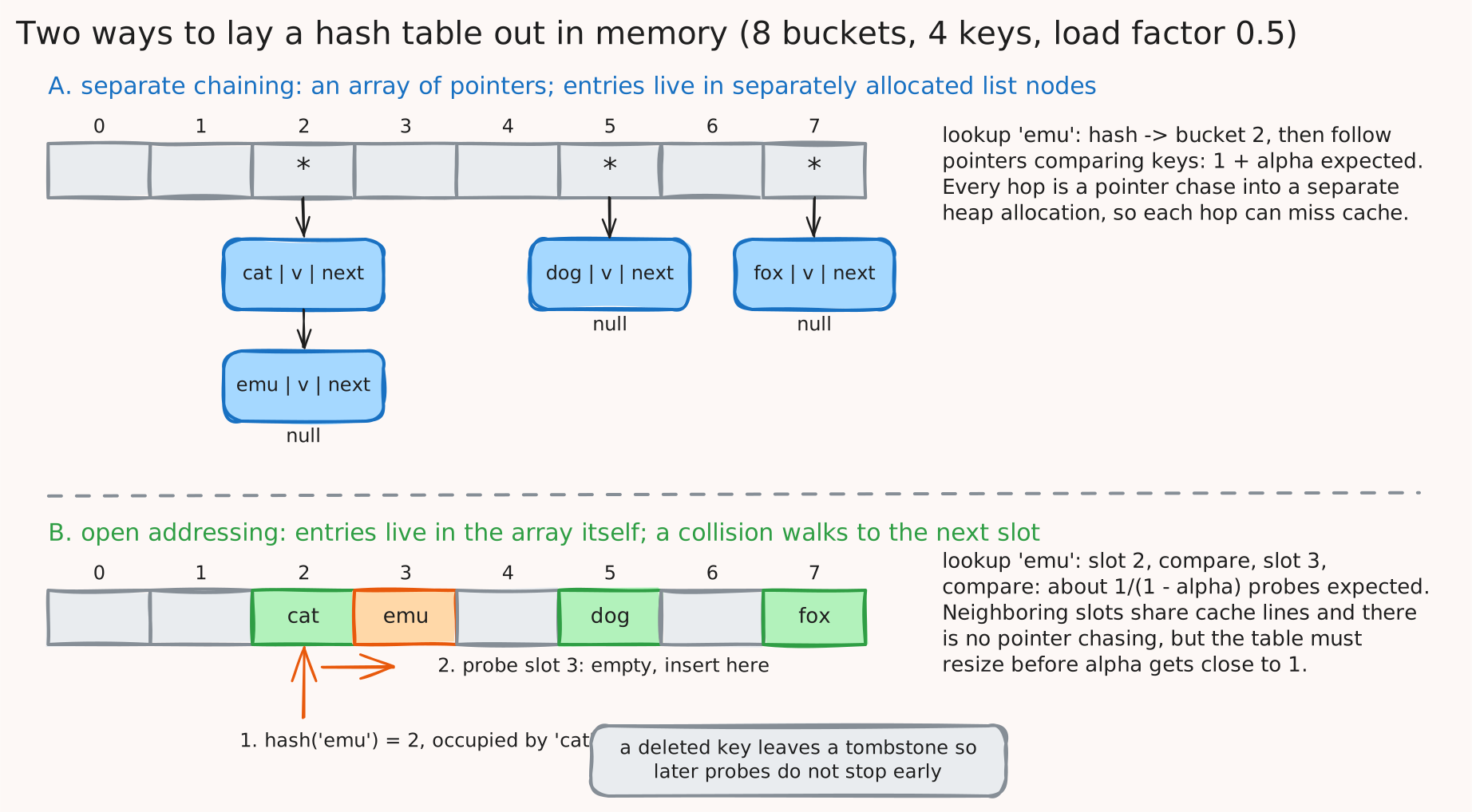
Separate chaining. The array holds \(m\) pointers, each to a linked list (or other small container) of the entries that hashed to that bucket. Collisions just extend the list. Insert appends to the list, lookup walks it comparing keys, delete unlinks a node. The array itself is small and fixed, and the entries live wherever the allocator put them.
Open addressing. The array holds the entries themselves, one per slot. On a collision, the insert probes other slots according to a fixed rule until it finds an empty one, and the lookup follows the same rule until it finds the key or an empty slot. Erickson describes the probe sequences that matter (Hashing notes, sections 5.8 and 5.9): linear probing tries \(h(x), h(x) + 1, h(x) + 2, \ldots\); quadratic probing tries \(h(x) + i^2\); double hashing steps by a second hash function. Deletion is the awkward case, because emptying a slot would break every probe sequence that passed through it, so a deleted slot is marked with a tombstone that lookups skip over and inserts may reuse.
| Separate chaining | Open addressing | |
|---|---|---|
| What the array holds | Pointers to lists of entries | The entries themselves |
| Collision handling | Append to the bucket’s list | Probe to another slot |
| Load factor \(\alpha = n/m\) | Can exceed 1 | Must stay below 1, in practice well below |
| Expected unsuccessful search | \(\Theta(1 + \alpha)\) | At most \(1/(1 - \alpha)\) with ideal probing |
| Memory | One pointer per bucket plus a node per entry | One slot per entry plus empty slots |
| Cache behavior | A pointer chase per hop | Consecutive slots, cache friendly (linear probing) |
| Deletion | Unlink a node | Tombstone |
| Degrades when | Lists get long | Slots cluster as \(\alpha \to 1\) |
The cache row is why modern implementations lean toward open addressing. Erickson makes the same observation about linear probing: it visits consecutive entries, so it has better cache performance than other strategies, and the clustering that hurts its probe count also means each access loads several nearby entries into the cache (Hashing notes, section 5.9).
Why O(1), exactly
The number that governs everything is the load factor, \(\alpha = n/m\): entries per bucket. Under the standard assumption that the hash function spreads keys uniformly (or is drawn from a universal family), the expected length of any one chain is \(\alpha\), so an unsuccessful search in a chained table costs one hash plus about \(\alpha\) comparisons, \(\Theta(1 + \alpha)\) expected (Erickson, Hashing notes, section 5.4). For open addressing with an ideal probe sequence, the expected number of probes in an unsuccessful search is at most \(1/(1 - \alpha)\) (section 5.8). That second formula is worth having in your head as a table, because it says exactly why open-addressed tables resize early:
| \(\alpha\) | \(1/(1 - \alpha)\) expected probes |
|---|---|
| 0.5 | 2 |
| 0.67 | 3 |
| 0.75 | 4 |
| 0.9 | 10 |
So \(O(1)\) means: as long as \(\alpha\) is held below a constant, the expected cost is a constant. The table holds \(\alpha\) below a constant by growing. When \(n\) crosses a threshold fraction of \(m\), allocate a new array of size \(2m\) and reinsert every entry. That reinsertion is \(O(n)\), which looks like it breaks the constant-time claim for that one insert, and this is where “amortized” earns its keep. Starting from an empty table and doubling each time it fills, the reinsertion work over \(N\) total inserts is
\[1 + 2 + 4 + \cdots + \tfrac{N}{2} + N \;<\; 2N\]so the total work for \(N\) inserts is under \(3N\) and the amortized cost per insert is \(O(1)\). Sedgewick states the general form for any resizing-array structure: from empty, any sequence of \(N\) operations takes time proportional to \(N\) in the worst case (Analysis of Algorithms), and the doubling-on-full, halving-at-one-quarter policy is the one he uses for resizing arrays (Bags, Queues, and Stacks). Java’s HashMap documents its version of the threshold: a default initial capacity of 16 buckets and a default load factor of 0.75 (HashMap javadoc).
Now the other half of the honest answer: when it is not O(1). The expected bound assumes the hash spreads keys. If every key lands in the same bucket, a chained table is a linked list and every operation is \(O(n)\); building a table of \(n\) such keys is \(O(n^2)\). That is not only a theoretical worst case. An attacker who knows the hash function can construct colliding keys on purpose, which is why CPython randomizes string hashing per process: hash randomization “is intended to provide protection against a denial-of-service caused by carefully chosen inputs that exploit the worst case performance of a dict construction, \(O(n^2)\) complexity”, and it is enabled by default (Python command line docs, PYTHONHASHSEED). Java takes the other route and changes the data structure under attack: a bucket whose chain grows past a threshold of 8 entries is converted from a list into a balanced tree, so the worst case per bucket becomes \(O(\log n)\) rather than \(O(n)\) (TREEIFY_THRESHOLD = 8 in HashMap.java, as of 2026-09-17).
So the complete answer to “why is a hash table lookup \(O(1)\)?” has four parts: the hash maps the key directly to an array index; the load factor is held below a constant by resizing; the resize cost amortizes to \(O(1)\) because the table doubles; and all of it is expected-case under a well-spread hash, with \(O(n)\) as the worst case that hash randomization and treeified buckets exist to prevent.
One concrete layout: the CPython dict
Textbook diagrams stop at “an array of buckets”. Here is what one real table looks like, because the interview question “how is it laid out in memory?” is easier to answer with a specific picture in mind. The facts below are from the header comment and constants in Objects/dictobject.c on CPython main as of 2026-09-17.
A CPython dict is open addressing, but the array of slots does not hold the entries. It is split in two:
-
dk_indices: the actual hash table, a sparse array of small integers. Each slot holds either the index of an entry in the second array, or \(-1\) for empty (DKIX_EMPTY), or \(-2\) for deleted (DKIX_DUMMY, the tombstone). The integer width scales with the table:int8while the table has at most 128 slots,int16up to \(2^{15}\),int32up to \(2^{31}\),int64beyond. -
dk_entries: a dense array of entries, each a (hash, key, value) triple, in insertion order. It is mostly append only, and its length is the usable fraction of the index table.
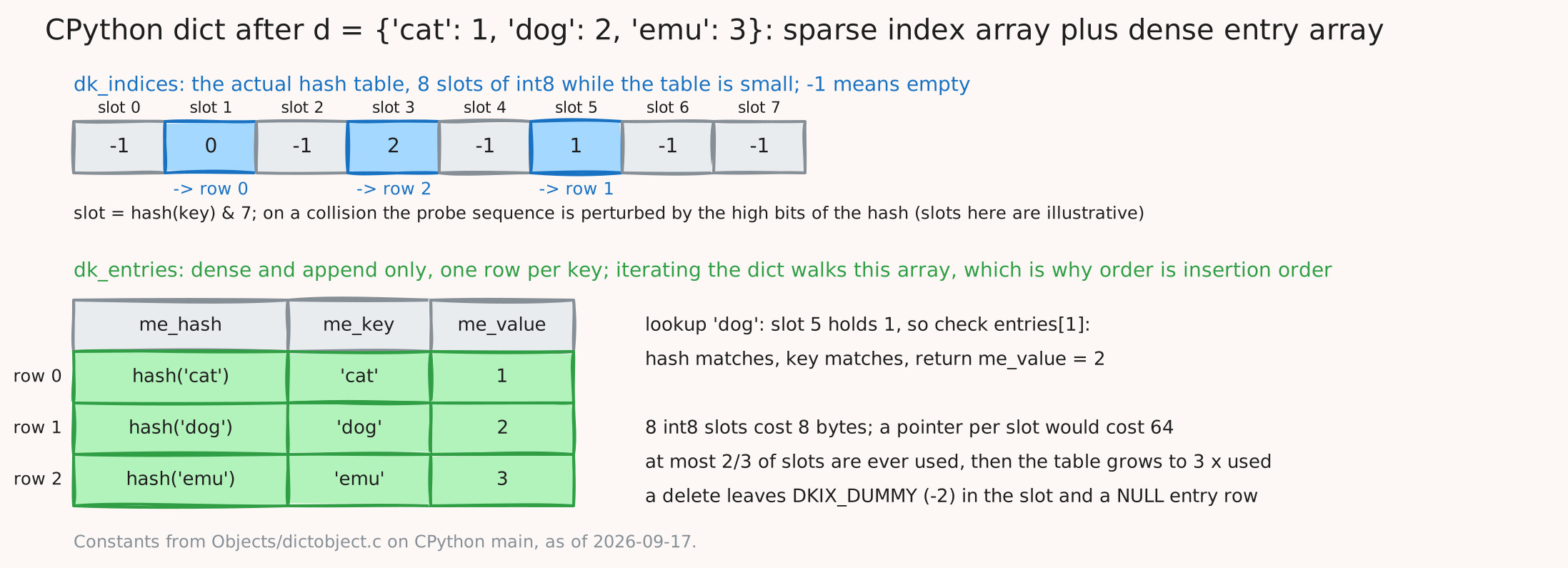
The constants that shape it (same source): the minimum table size is 8 (PyDict_MINSIZE), at most two thirds of the slots are ever used (USABLE_FRACTION(n) = (2n)/3), and when the table fills it grows to three times the number of live entries (GROWTH_RATE(d) = ma_used * 3). Collisions are resolved by a probe sequence that mixes in the high bits of the hash five at a time (PERTURB_SHIFT = 5), which is why the source comment can get away with very regular hash functions for integers. Three consequences worth knowing:
- Memory. A slot in the index array costs one byte in a small table, not a pointer. The sparse part of the structure is cheap, and the dense entries pack with no holes.
- Ordering. Iterating the dict walks
dk_entries, so iteration order is insertion order as a side effect of the layout. The compact layout landed in 3.6 (What’s New in Python 3.6) and Python made the ordering a language guarantee in 3.7 (What’s New in Python 3.7). - Deletion. A delete leaves a
DKIX_DUMMYin the index array and aNULLentry, so probe sequences still pass through, and the space is reclaimed on the next resize.
When to reach for something else
The question that follows “why \(O(1)\)?” is usually “so why would you ever use a tree?”.
| Hash table | Balanced search tree | |
|---|---|---|
| Lookup, insert, delete | \(O(1)\) expected, \(O(n)\) worst | \(O(\log n)\) worst case, guaranteed |
| Ordered iteration, min, max, range queries | Not supported | \(O(\log n)\) or \(O(\log n + k)\) for \(k\) results |
| Key requirements | Hashable, with a good hash | Comparable |
| Memory | Empty slots or per-node pointers | Two or three pointers per node |
| Predecessor and successor | No | Yes |
If you need the keys in order, or you need a hard worst-case bound, or your keys are naturally comparable and awkward to hash, the tree wins. Otherwise the hash table does.
References
- Jeff Erickson, Hashing notes (chaining, load factor, open addressing, probing)
- Python glossary, hashable
- Python data model,
__hash__ - Python command line, PYTHONHASHSEED and hash randomization
- What’s New in Python 3.6
- What’s New in Python 3.7
- CPython, Objects/dictobject.c
- Sedgewick and Wayne, Algorithms, Analysis of Algorithms
- Sedgewick and Wayne, Algorithms, Bags, Queues, and Stacks
- Java 21 HashMap javadoc
- OpenJDK, java/util/HashMap.java
Matrix Multiplication
The count
Take \(A\) of shape \(m \times k\) and \(B\) of shape \(k \times n\). The product \(C = AB\) has shape \(m \times n\), and each entry is a dot product of a row of \(A\) with a column of \(B\):
\[C_{ij} = \sum_{p=1}^{k} A_{ip} \, B_{pj}\]The inner dimension \(k\) has to match, because that is the length of the two vectors being dotted. If it does not, the product is not defined, and that is the whole story for “what if the shapes are wrong”: there is no cost to compute, the operation does not exist. Numpy will tell you so with a shape error.
The cost falls straight out of the formula. There are \(mn\) entries in \(C\), and each one costs \(k\) multiply-add pairs. So:
\[\text{multiply-adds} = m \cdot n \cdot k, \qquad \text{flops} = 2\,mnk\]The factor of two is the convention that a multiply and an add are separate floating point operations, which is how GPU peak numbers are quoted. The textbook version is the same statement with different letters: multiplying an \(m \times n\) matrix by an \(n \times p\) matrix takes \(mnp\) multiplications (Dasgupta, Papadimitriou, Vazirani, chapter 6.5). In code it is the triple loop, and the loop bounds are the count:
def matmul(A, B):
    m, k = len(A), len(A[0])
    k2, n = len(B), len(B[0])
    assert k == k2, "inner dimensions must match"
    C = [[0.0] * n for _ in range(m)]
    for i in range(m):            # m
        for j in range(n):        #   x n
            for p in range(k):    #     x k
                C[i][j] += A[i][p] * B[p][j]
    return C
When all three dimensions are the same \(n\), this is the familiar \(O(n^3)\). The answer to “what is the complexity of matrix multiplication?” is \(O(mnk)\), and \(O(n^3)\) is the special case where someone has told you the matrices are square.
Irregular shapes
The interview follow-up is “what happens when they are different sizes?”, and the answer has two levels. The first is that nothing changes: the count is \(mnk\) and you plug in the three numbers. The second, and the one worth showing you know, is that the ratio of work to data changes enormously with shape, and that ratio decides whether the multiply is fast.
The work is \(2mnk\) flops. The data is the three matrices: \(mk + kn + mn\) elements, times the bytes per element \(s\). Their ratio is the arithmetic intensity, the number the roofline model uses to decide whether a kernel is bound by compute or by memory bandwidth (the model is set out in the LLM inference systems post, and the original is Williams, Waterman, and Patterson):
\[I = \frac{2\,mnk}{s\,(mk + kn + mn)} \quad \text{flops per byte}\]Working through the shapes, with \(s = 4\) for fp32:
| Shape | Name | Flops | Elements moved | Intensity (fp32) | What it means |
|---|---|---|---|---|---|
| \(n \times n\) times \(n \times n\) | Square GEMM | \(2n^3\) | \(3n^2\) | \(n/6\); about 683 at \(n = 4096\) | Grows with \(n\); large square products are compute bound |
| \(m \times k\) times \(k \times 1\) | Matrix-vector | \(2mk\) | about \(mk\) | about \(0.5\) | Every weight is read once and used once; memory bound at any size |
| \(m \times 1\) times \(1 \times n\) | Outer product | \(2mn\) | about \(mn\) | about \(0.5\) | No reduction at all; memory bound |
| \(m \times k\) times \(k \times n\), \(m \gg k, n\) | Tall-skinny | \(2mnk\) | about \(mk + mn\) | about \(\frac{2nk}{4(k + n)}\), independent of \(m\) | Bounded by the small dimensions; a \(k = n = 64\) product tops out near 16 |
The intensity column is the number to reason with. A square product gets more compute per byte as it grows, which is why big GEMMs hit the compute roof. A matrix-vector product reads every element of the matrix once and does two flops with it, and no amount of cleverness changes that; it is bandwidth bound, full stop. This is the same fact that makes LLM decoding memory bound: a batch of one is a matrix-vector product against every weight matrix, and the fix (batching more tokens) is literally turning \(n = 1\) into \(n = B\) in the table above. The transformer block FLOPs post does that bookkeeping for a full layer.
Two further shape cases come up in practice:
- Batched. A stack of \(b\) independent products of shape \(m \times k\) by \(k \times n\) costs \(b \cdot 2mnk\). The batch dimension just multiplies through. Broadcasting a single \(B\) against \(b\) copies of \(A\) has the same flop count but reads \(B\) once, which raises the intensity.
- Non-conforming. If \(k\) does not match there is no product. If someone wants \(A B\) where the shapes are \(m \times k\) and \(n \times k\), what they mean is \(A B^\top\), and the count is still \(mnk\). In numpy the transpose is a view of the same memory, not a copy (ndarray.T).
Chains: the order matters
Matrix multiplication is associative but not commutative, so a chain \(ABC\) can be evaluated as \((AB)C\) or \(A(BC)\) and the answer is the same. The cost is not. The DPV textbook example makes the point with four matrices of shapes \(50 \times 20\), \(20 \times 1\), \(1 \times 10\), and \(10 \times 100\) (chapter 6.5). Counting \(mnk\) per product:
| Parenthesization | Cost computation | Multiplications |
|---|---|---|
| \(A \times ((B \times C) \times D)\) | \(20 \cdot 1 \cdot 10 + 20 \cdot 10 \cdot 100 + 50 \cdot 20 \cdot 100\) | 120,200 |
| \((A \times (B \times C)) \times D\) | \(20 \cdot 1 \cdot 10 + 50 \cdot 20 \cdot 10 + 50 \cdot 10 \cdot 100\) | 60,200 |
| \((A \times B) \times (C \times D)\) | \(50 \cdot 20 \cdot 1 + 1 \cdot 10 \cdot 100 + 50 \cdot 1 \cdot 100\) | 7,000 |
A factor of 17 between the worst and best order, on the same four matrices. The intuition: \(B\) is \(20 \times 1\), so \(AB\) is a skinny \(50 \times 1\) column and \(CD\) is a skinny \(1 \times 100\) row, and multiplying skinny things is cheap. The best order squeezes through the small dimension early. DPV also note that greedy (always do the cheapest available product next) picks the second row, not the third, so the problem needs actual optimization.
The standard solution is dynamic programming. For matrices \(A_1, \ldots, A_n\) with dimensions \(m_0 \times m_1, m_1 \times m_2, \ldots, m_{n-1} \times m_n\), let \(C(i, j)\) be the cheapest cost of computing \(A_i \cdots A_j\). The last multiplication splits the chain at some \(k\), so
\[C(i, j) = \min_{i \le k < j} \left\{ C(i, k) + C(k + 1, j) + m_{i-1} \, m_k \, m_j \right\}, \qquad C(i, i) = 0\]There are \(O(n^2)\) subproblems and each takes \(O(n)\) to evaluate, so the whole thing is \(O(n^3)\) in the number of matrices, which is trivial next to the multiplications it saves (DPV, chapter 6.5). The practical version of this fact is in the einsum post: contracting three or more tensors in the wrong order can change the flop count by orders of magnitude, and np.einsum does not optimize the order unless you ask it to.
Below cubic, in theory
The triple loop is \(\Theta(n^3)\), and for a long time that was assumed to be optimal. Strassen’s 1969 result (Gaussian Elimination is not Optimal) broke it with a divide-and-conquer trick: split each \(n \times n\) matrix into four \(n/2 \times n/2\) blocks, and instead of the eight block products the obvious recursion needs, compute seven cleverly chosen ones and recover the answer with additions. The recurrence becomes
\[T(n) = 7 \, T(n/2) + O(n^2) \quad \Longrightarrow \quad T(n) = O(n^{\log_2 7}) \approx O(n^{2.807})\]which is the “leaves dominate” case of the recursion tree, exactly as \(8T(n/2) + O(n^2)\) gives \(n^{\log_2 8} = n^3\) for the naive split. The exponent has kept dropping since, through Coppersmith and Winograd and a run of laser-method refinements; the current bound on the matrix multiplication exponent \(\omega\), per the abstract of Alman, Duan, Vassilevska Williams, Xu, Xu, and Zhou as of 2026-09-17, is \(\omega < 2.371177\). The lower bound is \(\omega \ge 2\), since you have to at least read the input.
Two honest caveats for the interview. First, to my knowledge none of the sub-cubic algorithms past Strassen are used in practice: the constants hidden in the big-O are large enough that they only overtake the cubic algorithm at sizes no machine holds, and even Strassen is a niche choice. Second, and more important, the real speedups in practice come from the bytes, not the flops. A production GEMM is still \(2mnk\) flops; what makes it fast is blocking the loops so that a tile of \(A\) and \(B\) stays in cache or shared memory while it is reused, which raises the arithmetic intensity toward the compute roof. That is the subject of the GEMM kernel optimization notes and the CUTLASS WGMMA notes, and it is where the \(O(mnk)\) answer stops being the interesting part.
References
- Dasgupta, Papadimitriou, Vazirani, Algorithms, chapter 6 (section 6.5, chain matrix multiplication)
- Williams, Waterman, Patterson, Roofline: An Insightful Visual Performance Model, Berkeley tech report
- Strassen, Gaussian Elimination is not Optimal, Numerische Mathematik 1969
- Alman, Duan, Vassilevska Williams, Xu, Xu, Zhou, More Asymmetry Yields Faster Matrix Multiplication
- numpy, ndarray.T
- Jeff Erickson, Algorithms, chapter 1: Recursion (recursion tree cases)
Test Yourself
Answers are short on purpose. If one is not obvious, the section it came from has the derivation.
Foundations
1. Expected, amortized, worst case: which one does “hash table insert is O(1)” mean? Expected (over the hash spreading keys) and amortized (over a sequence, absorbing resizes). The worst case for a single insert is \(O(n)\).
2. Solve \(T(n) = 2T(n/2) + n\), \(T(n) = T(n-1) + n\), and \(T(n) = 7T(n/2) + n^2\). \(O(n \log n)\) (all levels equal), \(O(n^2)\) (a chain, sum of \(n + (n-1) + \cdots\)), \(O(n^{\log_2 7}) \approx O(n^{2.807})\) (leaves dominate).
3. Roughly how many operations is \(n \log_2 n\) for a million elements, and how does that compare to \(n^2\)? About \(2 \times 10^7\) against \(10^{12}\). The log factor is 20; the quadratic is fifty thousand times worse.
Sorting
1. Why can no comparison sort beat \(n \log n\)? A decision tree that sorts must have at least \(n!\) leaves, one per output permutation, so its depth is at least \(\log_2(n!) = \Omega(n \log n)\) by Stirling. Depth is the worst-case comparison count.
2. Merge sort’s recurrence and the two costs it implies. \(T(n) = 2T(n/2) + O(n)\), so \(\Theta(n \log n)\) time in every case, plus \(O(n)\) extra space for the merge buffer.
3. Quicksort with the last element as pivot on an already sorted array: what happens and why? Every partition puts the pivot at an end, so the recurrence is \(T(n) = T(n-1) + O(n)\) and the run is \(O(n^2)\). Sorted input is the worst case, not the best.
4. Does median-of-three fix the quicksort worst case? What does? No: an adversary can still force a split of 1 against \(n - 2\), which is still \(O(n^2)\). A uniformly random pivot gives \(O(n \log n)\) with high probability on every input.
5. Quicksort does about 39 percent more comparisons than merge sort on average. Why is it usually faster anyway? It is in place, its partition is a sequential scan, and it moves far less data; merge sort copies every element at every level into a buffer. The compares are not the cost, the bytes are.
6. State the Lomuto partition invariant. With pivot at the end, scan pointer \(j\), and boundary \(i\): everything in \(A[lo..i]\) is at most the pivot, everything in \(A[i+1..j-1]\) is greater, and \(A[j..hi-1]\) is unscanned.
7. Which sort do you pick for a linked list, for stability, for guaranteed \(n \log n\) in place, and for nearly sorted data? Merge sort, merge sort (or Timsort), heapsort, insertion sort (or Timsort, which is linear on it).
8. What does Python’s sorted actually run, and what is its worst case? Timsort: run detection, binary insertion sort to extend short runs, merging of runs. \(O(n \log n)\) worst case, \(O(n)\) on already ordered data, stable.
9. How does radix sort get under \(n \log n\), and when is it actually a win? It never compares keys; each pass is a counting sort on one digit, so the total is \(O(d(n + b))\). It wins when \(d\) (digits) is smaller than \(\log n\), which means large arrays of small fixed-width keys.
10. Why must each radix sort pass be stable? Sorting on digit \(i\) must keep the order established by digits \(0\) through \(i - 1\) for ties, otherwise the earlier passes are wasted.
Hash tables
1. Walk through a lookup, from key to value. Hash the key to an integer, reduce it modulo the table size to an index, go to that bucket, compare stored keys until a match (chaining: walk the list; open addressing: follow the probe sequence until the key or an empty slot).
2. What two properties must a key have, and why can a Python list not be one? Its hash must not change during its lifetime, and equal keys must hash equal. A list can be mutated after insertion, which would leave it in a bucket its new hash no longer points to.
3. Chaining versus open addressing: where do the entries live, and which is more cache friendly? Chaining keeps entries in separately allocated list nodes reached by pointer; open addressing keeps them in the array itself. Open addressing with linear probing is more cache friendly because probes touch consecutive slots.
4. Define the load factor and give the expected cost of an unsuccessful search in both layouts. \(\alpha = n/m\). Chaining: \(\Theta(1 + \alpha)\). Open addressing with ideal probing: at most \(1/(1 - \alpha)\), which is 4 probes at \(\alpha = 0.75\) and 10 at \(0.9\).
5. Resizing costs \(O(n)\). How is insert still \(O(1)\)? Amortized: doubling means the total reinsertion work over \(N\) inserts is \(1 + 2 + 4 + \cdots < 2N\), so the average per insert is constant.
6. When is a hash table \(O(n)\) per operation, and what do real implementations do about it? When keys collide into one bucket, whether by bad luck or by an attacker constructing them. CPython randomizes string hashes per process; Java converts a bucket with more than 8 entries into a balanced tree.
7. Why does a deleted slot in an open-addressed table need a tombstone? Blanking the slot would terminate every probe sequence that passed through it, hiding keys that were inserted past it. The tombstone tells lookups to keep going and inserts that the slot is reusable.
8. How is a CPython dict laid out, and why does it iterate in insertion order? A sparse index array of small integers (the hash table) pointing into a dense, append-only array of (hash, key, value) entries. Iteration walks the dense array, so the order is insertion order.
9. When would you use a balanced tree instead? When you need ordered iteration, range queries, min or max, predecessor or successor, or a guaranteed \(O(\log n)\) worst case rather than an expected \(O(1)\).
Matrix multiplication
1. Cost of \(A\) (\(m \times k\)) times \(B\) (\(k \times n\)), and why. \(mnk\) multiply-adds, \(2mnk\) flops: \(mn\) output entries, each a dot product of length \(k\). \(O(n^3)\) is the square special case.
2. What if the shapes do not conform? The product is undefined; there is nothing to compute. If the intent was \(AB^\top\), the count is still \(mnk\) and the transpose is free.
3. A \(4096 \times 4096\) square product and a \(4096 \times 4096\) matrix-vector product have very different speeds per flop. Why? Arithmetic intensity: \(2n^3 / (3n^2 \cdot 4)\) bytes gives about 683 flops per byte for the square product, against about 0.5 for the matrix-vector product, which reads every weight once and uses it twice. One is compute bound, the other is bandwidth bound.
4. \(ABCD\) with shapes \(50 \times 20\), \(20 \times 1\), \(1 \times 10\), \(10 \times 100\): best and worst order? \((AB)(CD)\) at 7,000 multiplications against \(A((BC)D)\) at 120,200. Squeeze through the dimension of size 1 first. The general problem is an \(O(n^3)\) dynamic program over the split point.
5. Strassen’s recurrence and exponent, and why nobody uses the algorithms after it. \(T(n) = 7T(n/2) + O(n^2) = O(n^{\log_2 7}) \approx O(n^{2.807})\). The later ones (currently \(\omega < 2.371177\)) have constants so large they never win at feasible sizes; practical speed comes from blocking for cache, not from fewer flops.
Wrapping up
The three questions look unrelated, but the answers share one habit. Sorting: count comparisons, then notice that merge sort’s compares are cheap and its copies are not, and that quicksort’s compares are more numerous and its bytes fewer. Hash tables: the array index makes lookup constant, the load factor keeps it constant, doubling makes resizing constant on average, and the layout in memory (pointers to nodes, or entries in the array, or CPython’s split into a sparse index and a dense entry array) decides how many cache lines a lookup touches. Matrix multiplication: \(mnk\) is the flop count, and the shape decides the byte count, which is the number that actually predicts speed.
Count the operations, then count the bytes. The second number usually explains the first.
If you find a mistake anywhere in here, please let me know and I’ll fix it.