LLM Inference Systems - From the Roofline to vLLM Internals
Hello all. This post is a top-to-bottom tour of LLM inference systems: what happens between a request arriving at a serving engine and tokens streaming back out, and why the systems are shaped the way they are.
The angle throughout is performance. Almost every design decision in a modern inference engine traces back to one fact: generating a token is cheap on arithmetic and expensive on memory traffic. Once that fact is internalized, the whole stack, paged KV caches, continuous batching, speculative decoding, disaggregated prefill, stops looking like a pile of unrelated tricks and starts looking like one idea applied at different layers. So we’ll build the performance model first, with real numbers, and then walk the stack with that model in hand.
Concepts come first, but everything is anchored in a real engine: vLLM’s V1 architecture. It’s open source, it’s the engine whose design documents actually explain their reasoning, and pointing at the file that implements an idea keeps the discussion honest. One convention up front: vLLM moves fast, so every vLLM file path, symbol name, and default quoted here was verified against main as of 2026-08-21, and I’ve kept that stamp next to the claims most likely to move. Papers and official docs are linked inline where each claim is made, and each major section ends with its references.
The plan:
- The problem: autoregressive generation, the KV cache, and the two phases
- The numbers that drive everything: GPU specs, the roofline, and three formulas
- Metrics: TTFT, ITL, TPOT, goodput, and how vLLM measures them
- Batching: static, continuous, chunked
- KV cache management and PagedAttention
- Prefix caching
- Scheduling in vLLM V1
- Speculative decoding
- Distributed inference: TP, PP, DP, EP
- Disaggregated prefill and KV transfer
- Attention kernels
- Quantization and MoE
- The engine at runtime: processes, CUDA graphs, torch.compile, sampling
- Test yourself: a question bank over everything above
I’m assuming you’re comfortable with what a transformer is and does; we won’t re-derive attention here. This is a long one, but the sections build on each other in order, and the question bank at the end is there so you can check what stuck.
Let’s get started.
The Problem
Autoregressive generation
An LLM generates text one token at a time, and each new token depends on all the tokens before it. That single property sets up everything that follows. Producing \(m\) output tokens requires at least \(m\) sequential forward passes; there is no way to parallelize across the output positions of a single request, because position \(t+1\)’s input includes position \(t\)’s output.
It has a second consequence that is easy to miss and that a serving engine cannot ignore: output length is unknown at admission time. When a request arrives, the engine does not know whether it will generate 5 tokens or 5,000, which means it cannot know how long the request will occupy memory or how much of it. Every memory-management decision in this post is downstream of that uncertainty. A generation ends when the model emits a stop condition; in vLLM the recorded finish reasons are stop (EOS token or stop string), length (hit the token limit), and abort (docs/design/metrics.md).
The KV cache
Inside each transformer layer, attention needs the key and value projections of every token in the prefix. Recomputing those for the whole prefix on every step would make step \(t\) cost \(O(t)\) redundant work, so instead the engine stores them: the KV cache holds the K and V vectors for every token, at every layer, for every live request, and each decode step appends one more token’s worth (Pope et al., kipply’s inference arithmetic). This is the classic time-for-space trade, and the space is substantial; we’ll put exact numbers on it in the next section, but for a sense of scale, a single 8K-token request on Llama 3 70B carries 2.5 GiB of cache.
The KV cache is state. That one word is why inference serving is a systems problem and not just a kernels problem: requests arrive, grow a variable-sized allocation at an unpredictable rate, and leave at an unpredictable time, and the engine has to pack them into fixed GPU memory without fragmenting it or running out.
Two phases, one cache
Serving one request has two distinct phases, and they could hardly be more different:
| Prefill | Decode | |
|---|---|---|
| Input per step | the whole prompt (\(P\) tokens) | 1 token per sequence |
| Purpose | populate the KV cache, emit the first token | extend the KV cache, emit the next token |
| Arithmetic intensity | \(\approx P\) FLOP/byte | \(\approx B\) (batch size) FLOP/byte |
| Regime | compute-bound | memory-bound until \(B\) nears the ridge point |
Prefill processes the entire prompt in one forward pass. All \(P\) tokens flow through the model together, every matrix multiply is fat, and the GPU’s compute units are the bottleneck. Decode processes one token per sequence per step. The matrix multiplies are skinny (one row per sequence), and the bottleneck flips: the step spends its time streaming the model’s weights out of GPU memory, not doing math on them. vLLM’s own docs use exactly this framing, compute-bound prefill and memory-bound decode (docs/configuration/optimization.md).
Why the flip happens is worth spelling out, because it’s the load-bearing fact of the whole post. Each forward pass must read every weight of the model from GPU memory, whether it processes 1 token or 10,000. Prefill amortizes that weight read over \(P\) tokens of useful work. A decode step amortizes it over 1 token per sequence, so the only way to amortize it at all is batching: with \(B\) sequences decoding together, one weight read serves \(B\) tokens. That’s the origin of the arithmetic-intensity row in the table (made precise in the next section): prefill’s intensity scales with prompt length, decode’s with batch size.
There’s a catch inside the batching remedy, though. Weight reads amortize over the batch, but KV cache reads do not: each sequence attends over its own cache, so KV traffic grows with \(B \times \text{context length}\) while weight traffic stays flat. Per decode step the engine moves roughly the weight bytes plus \(B \times n \times \text{KV-bytes-per-token}\) for \(B\) tokens of output. At long contexts the KV term dominates, which is why long-context decode stays memory-bound even at batch sizes that would otherwise saturate compute, and why so much of this post is about making KV bytes smaller, shareable, or better placed.
The engine’s inner loop
With those pieces named, a serving engine’s job is easy to state. It maintains a pool of in-flight requests, and it loops: pick which requests run this step, allocate KV memory for the tokens about to be computed, run one forward pass for the whole batch, sample one token per sequence, hand back outputs, repeat. Everything in this post lives inside that loop: the metrics measure it, the scheduler drives it, the KV manager feeds it, and the kernels are what it launches.
References
- Efficiently Scaling Transformer Inference - Pope et al.
- Transformer Inference Arithmetic - kipply
- vLLM optimization docs
- vLLM metrics design doc
The Numbers That Drive Everything
Before any mechanisms, the numbers. This section is the reference the rest of the post leans on: the hardware, the one performance model worth internalizing, and three formulas. None of it is hard, but the later sections quote these figures constantly, so it pays to have them in one place. All figures were verified against the linked sources, accessed 2026-08-21.
The hardware
The two GPUs that anchor every example in this post:
| A100 SXM 80GB | H100 SXM | |
|---|---|---|
| Memory | 80 GB HBM2e | 80 GB HBM3 |
| Bandwidth | 2,039 GB/s | 3.35 TB/s |
| BF16 dense | 312 TFLOPS | ~1000 TFLOPS |
| BF16 “with sparsity” | 624 TFLOPS | 1,979 TFLOPS |
| FP8 dense | n/a (no FP8 tensor cores) | ~2000 TFLOPS |
| SMs | 108 | 132 |
| L2 cache | 40 MB | 50 MB |
| Ridge point (dense BF16 / bandwidth) | ~153 FLOP/B | ~300 FLOP/B |
Sources: NVIDIA A100 page, NVIDIA H100 page, Hopper architecture in-depth (which gives the H100 SM count, L2 size, and dense TFLOPS; its table rounds to 1000/2000), Ampere architecture in-depth (A100 SMs and L2). One trap worth flagging: marketing pages quote the “with sparsity” number, which assumes 2:4 structured sparsity in the weights. Dense workloads, which is what LLM inference is, get half of it. When someone quotes 1,979 TFLOPS for an H100, the usable number is ~1000.
A quick sketch of the machine behind the table, since the vocabulary recurs. A GPU is an array of streaming multiprocessors (SMs); work launches as a grid of thread blocks, blocks are assigned to SMs, and threads execute in warps of 32 (SIMT). Each H100 SM has 256 KB of registers and 256 KB of combined shared memory and L1 (of which up to 228 KB is configurable as shared memory); chip-wide sit the 50 MB L2 and the 80 GB of HBM3. Occupancy is “the ratio of active warps per multiprocessor to the maximum number of warps” (CUDA Best Practices Guide), and it matters because it’s the GPU’s latency-hiding mechanism: when one warp stalls on a memory access, the SM simply issues from another resident warp, so having many warps resident keeps the SM busy through stalls. Hopper also added three features worth knowing by name: TMA (Tensor Memory Accelerator), a per-SM DMA engine for asynchronous bulk copies between global and shared memory; thread block clusters with distributed shared memory, letting co-scheduled blocks on different SMs access each other’s shared memory; and FP8 tensor cores (E4M3 and E5M2 formats), which halve storage per element and double throughput relative to FP16/BF16 (Hopper in-depth).
The roofline
One model organizes everything: the roofline (Williams, Waterman, Patterson, CACM 2009). Define a kernel’s arithmetic intensity as the FLOPs it performs per byte it moves from DRAM:
\[I = \frac{\text{FLOPs}}{\text{bytes moved}}\]Then the performance it can attain is capped by whichever binds first, memory bandwidth or peak compute:
\[\text{attainable FLOP/s} = \min(\text{peak FLOP/s},\; I \times \text{bandwidth})\]The crossover is the ridge point, peak FLOP/s divided by bandwidth. For H100 dense BF16 that’s roughly \(10^{15} / 3.35 \times 10^{12} \approx 300\) FLOP per byte. Below the ridge a kernel is memory-bound: the compute units are starved, and optimizing the math does nothing; the only lever is moving fewer bytes (fuse kernels, shrink the dtype, batch more work per byte). Above the ridge it’s compute-bound, and the levers flip: tensor core utilization, occupancy, scheduling.
Now map LLM inference onto it, and the two-phase table from the previous section becomes quantitative:
- Decode has \(I \approx B\): a batch of \(B\) sequences does \(B\) tokens of work per weight read. On an H100 that means decode is memory-bound until batch size approaches ~300, and at, say, batch 64 the attainable fraction of peak is roughly \(64/300 \approx 21\%\). In practice the crossover sits even higher than 300, because the KV-read traffic that grows with batch and context keeps adding bytes to the denominator.
- Prefill has \(I \approx P\), the prompt length. Any realistic prompt puts it well above the ridge: prefill is compute-bound almost by construction.
- Elementwise ops (norms, activations, RoPE) have \(I = O(1)\): a few FLOPs per element read and written, independent of size. Alone, they are hopelessly memory-bound, which is the entire case for kernel fusion: fused into a neighboring op, they ride on bytes that were already moving. (This is the same accounting that makes a standalone LayerNorm memory-bound; I went through that op’s arithmetic in the LayerNorm and RMSNorm post.)
One more roofline remark that will matter in the quantization section: the dtype moves both lines. FP8 doubles peak FLOP/s (the roof rises) and halves the bytes per element (the kernel’s intensity rises). Both shifts push a kernel toward compute-bound.
The models
The Llama 3 family is the running example, because its architecture table is public and its sizes span the practical range (Llama 3 paper, Table 3):
| 8B | 70B | 405B | |
|---|---|---|---|
| Layers \(L\) | 32 | 80 | 126 |
| \(d_{model}\) | 4096 | 8192 | 16384 |
| Q heads | 32 | 64 | 128 |
| KV heads | 8 | 8 | 8 |
| head_dim | 128 | 128 | 128 |
| FFN dim | 14336 | 28672 | 53248 |
| Vocab | 128K | 128K | 128K |
Notice the KV-heads row: 8 across the whole family. That’s grouped-query attention (GQA), and it exists precisely to shrink the KV cache; the formula below shows by how much.
Formula 1: KV bytes per token
\[\text{KV bytes per token} = 2 \times L \times H_{kv} \times d_{head} \times b\]where the leading 2 counts K and V, \(H_{kv}\) is the number of KV heads, and \(b\) is bytes per element (kipply). Running the Llama 3 numbers at bf16 (\(b = 2\)):
| Model | Per token | At 8K context |
|---|---|---|
| 8B | \(2 \cdot 32 \cdot 8 \cdot 128 \cdot 2\) = 128 KiB | 1.0 GiB |
| 70B | \(2 \cdot 80 \cdot 8 \cdot 128 \cdot 2\) = 320 KiB | 2.5 GiB |
| 405B | \(2 \cdot 126 \cdot 8 \cdot 128 \cdot 2\) = 504 KiB | 4.0 GiB |
These are the numbers to keep loaded. A single long-context request on the 70B model carries gigabytes of state, and note what the formula does not contain: the number of query heads. GQA is why: 64 query heads share 8 KV heads on the 70B model, an 8x saving already baked in. With full multi-head attention (\(H_{kv} = 64\)), the 70B figure would be 2.5 MiB per token and 20 GiB per 8K request, which is the difference between a GPU holding a healthy batch of requests in cache and holding a handful.
Formula 2: FLOPs per token
\[\text{FLOPs per token} \approx 2N \;+\; 2 \, L \, n_{ctx} \, d_{model}\]This is Kaplan et al., Eq. 2.2, and both terms are worth deriving rather than memorizing.
The \(2N\) term. Start from the general matmul count: multiplying an \(m \times k\) matrix by a \(k \times n\) matrix costs \(2mnk\) FLOPs, the 2 counting the multiply and the add of each multiply-accumulate. A single token passing through a linear layer is the \(m = 1\) case: a \(1 \times k\) row times a \(k \times n\) weight matrix costs \(2kn\) FLOPs, and \(kn\) is exactly the number of parameters in that weight matrix. So one token through one linear layer costs 2 FLOPs per parameter, and since a forward pass is one trip through every weight matrix in the model (the QKV and output projections, the FFN matrices, all \(L\) layers of them), the totals just add up: roughly 2 FLOPs per parameter overall, hence \(2N\). If you want the op-by-op ledger behind this, block by block with the bytes counted too, I’ve worked through it in the transformer block accounting post.
What \(N\) is. \(N\) is the parameter count excluding the embedding table, and the exclusion has a mechanical justification: the input embedding is a table lookup, not a matmul, so its parameters contribute zero FLOPs. The output side is different, and worth being precise about since it’s a common point of confusion: the final logits projection (hidden state times the \(d_{model} \times V\) unembedding matrix) is a real matmul. The \(\approx\) absorbs it because it’s one matrix against the \(L\) layers’ worth in \(N\): for Llama 3 8B it’s \(2 \cdot 4096 \cdot 128256 \approx 1.1\) GFLOP per token against \(2N \approx 16\) GFLOP, about 7%, and the fraction shrinks as models grow (about 1.5% at 70B).
The attention term. Attention against the cached context is the one part of the forward pass that is not a multiply through a fixed weight matrix; its operand is the KV cache, and its cost grows with context. Per layer, the new token’s query is dotted against all \(n_{ctx}\) cached keys and the resulting weights are applied to the \(n_{ctx}\) values, work proportional to \(n_{ctx} \, d_{model}\); Kaplan’s accounting puts the total at \(2 \, L \, n_{ctx} \, d_{model}\) per token. It stays small until contexts get long: at 8K context on Llama 3 8B it’s \(2 \cdot 32 \cdot 8192 \cdot 4096 \approx 2.1\) GFLOP against the 16 GFLOP of \(2N\), about 13%, but it scales linearly with \(n_{ctx}\) while \(2N\) stays fixed.
And the \(6N\) you’ll see quoted for training. Same \(N\), different pass structure. Training costs roughly \(6N\) per token: the \(2N\) forward, plus a backward pass that costs about twice the forward, because each layer’s backward computes two matmul-shaped quantities, the gradient with respect to the weights and the gradient with respect to the input, each about a forward’s worth of work. (Those are exactly the outer-product and transposed-matmul shapes derived in the MLP forward and backward post.) Inference has no backward pass, so it’s the \(2N\) forward only.
Formula 3: the decode floor
This is the punchline the previous two set up. A decode step must read every weight byte, so, however good the kernels are:
\[\text{minimum decode step time} = \frac{\text{weight bytes}}{\text{memory bandwidth}}\]Worked example, Llama 3 8B in bf16 on one H100: 16 GB of weights over 3.35 TB/s gives
\[\frac{16 \times 10^9}{3.35 \times 10^{12}} \approx 4.8 \text{ ms per step}\]so single-stream decode is capped at roughly 210 tokens/s regardless of kernel quality. Now compare the arithmetic for that same step: \(2N = 16 \times 10^9\) FLOPs at \(10^{15}\) FLOP/s is about 16 µs, roughly 300x less than the memory time. The compute is essentially free; the step is the weight read. Every decode-latency technique in this post, batching, speculative decoding, tensor parallelism, quantization, is an attack on this one number: more useful tokens per weight read, or fewer weight bytes per read, or the read split across more GPUs.
Constants and defaults worth pinning
- Bytes per element: bf16/fp16 = 2, fp8/int8 = 1, int4 = 0.5.
- Weights at bf16 are roughly 2 bytes per parameter: the 8B model is 16 GB, 70B is 140 GB, 405B is 810 GB, before any KV cache, activations, or CUDA context. The 70B model doesn’t even fit on one 80 GB GPU; that observation is where the distributed section starts.
- vLLM defaults, from
vllm/config/cache.pyas of 2026-08-21:gpu_memory_utilization = 0.92(older docs say 0.9; the current code says 0.92), and a KV block size of 16 tokens (CacheConfig.DEFAULT_BLOCK_SIZE, applied when unset; platform or attention-backend preferences can override it,vllm/platforms/interface.py). Both matter in the KV cache section.
Why re-read the weights every step at all?
A fair objection to formula 3, and a question worth settling before moving on: the weights never change during inference, so why does every decode step pay to “read” them again? Can’t they just stay where they are?
They do stay where they are, in HBM; nothing re-uploads them from the CPU between steps. The read the floor charges is a different trip: from HBM to the compute units. Arithmetic happens in registers on the SMs, and the total on-chip storage, the 50 MB L2 plus each SM’s registers and shared memory, adds up to roughly 100 MB on an H100, against 16 GB of weights for even the small model. The weights physically cannot live next to the ALUs. So each layer’s matrices must stream on-chip, get used, and be overwritten by the next layer’s matrices, every single forward pass; “keeping the weights fixed” is exactly what already happens, and it doesn’t help, because the cost was never re-loading them onto the GPU, it was moving them across the last few centimeters. Caches don’t rescue this either: within one batch-1 decode step each weight is touched exactly once, and a value used once gains nothing from any cache tier. The only reuse available is across sequences in the same step, which is precisely what batching exploits.
Framed this way, the remedies from the rest of the post sort themselves: get more tokens out of each streaming pass (batching, speculative decoding), make the stream smaller (weight quantization), or split the stream across more HBM stacks in parallel (tensor parallelism). That’s the whole menu, and it’s the roofline’s memory-bound prescription, reduce or amortize bytes, applied to the one byte stream that can’t be skipped.
References
- NVIDIA A100 page, NVIDIA H100 page
- NVIDIA Hopper architecture in-depth, NVIDIA Ampere architecture in-depth
- CUDA C++ Best Practices Guide
- Roofline: An Insightful Visual Performance Model - Williams, Waterman, Patterson
- The Llama 3 Herd of Models
- Scaling Laws for Neural Language Models - Kaplan et al.
- Transformer Inference Arithmetic - kipply
Metrics
Before any more machinery, we need to fix what “fast” means. Every metric here is one of two kinds. Latency is one request’s experience: how long did this user wait. Throughput is the operator’s aggregate: how much work the whole system completes per second. The two pull against each other, and this section is about measuring each honestly.
One piece of vocabulary first: latency is a distribution over many samples, not a number, and p99 names the value that 99% of samples fall below (so p99 ITL = 200 ms means 1 gap in 100 was worse than that). Serving is judged at p99 rather than the mean because a request generating 500 tokens samples the gap distribution 500 times: even a 1-in-100 stall hits essentially every long request, and the user feels the freeze, not the average. That is why the targets later in this section are stated at percentiles.
The definitions:
| Metric | Stands for | Definition | What to watch |
|---|---|---|---|
| TTFT | time to first token | request sent to first token received | queueing plus prefill; client-side it also includes tokenization |
| ITL | inter-token latency | gap between consecutive tokens | the tail (p99) exposes prefill insertions and preemptions |
| TPOT | time per output token | \((\text{E2EL} - \text{TTFT}) / (\text{output tokens} - 1)\) | a per-request average; hides stalls |
| E2EL | end-to-end latency | request sent to last token | \(= \text{TTFT} + \sum \text{ITL}\) |
| Throughput | tokens/s or requests/s completed | meaningless without a latency constraint | |
| Goodput | requests/s meeting all stated SLOs | the comparable headline number (DistServe) |
ITL versus TPOT
These two sound interchangeable and are not. ITL is a sample per decode step: every gap between consecutive tokens is one measurement, so ITL has a distribution and a meaningful p99. TPOT is a per-request mean: total decode time divided by tokens generated. If a request stalls once for 800 ms mid-generation, that stall is one enormous ITL sample, while TPOT smears it across a few hundred tokens and barely moves. When hunting scheduling pathologies, ITL p99 is the metric that talks.
And the classic pathology to keep in mind: admitting a prompt helps that request’s TTFT and hurts everyone else’s ITL, because its prefill tokens ride in the same forward pass as the in-flight decodes and stretch the step for all of them. Every scheduler decision in this post sits somewhere on that trade-off.
Tokens/s versus requests/s
The throughput row lists two units because they answer different questions. Tokens/s counts the engine’s actual work (a 900-token generation is 100x the work of a 9-token one, and is weighted accordingly), which makes it the unit for comparing engines and kernels. Requests/s is what capacity planning buys: how many users one replica serves. Converting between them requires the workload’s average tokens per request, so the two agree only on a fixed workload. One convention to check in any benchmark: whether “tokens” means output tokens only or prompt plus output; both get reported, and on prefill-heavy workloads the difference is large.
Goodput
Raw throughput has a flaw that makes benchmark headlines misleading: any engine can buy tokens/s with batch size, at the cost of latency. One decode step reads the weights once and yields one token per sequence, so a bigger batch means more tokens per step; but the step also gets slower as the batch grows, so every user’s ITL worsens at the same time (a decoding user gets exactly one token per step, so their ITL is the step time, and each added sequence makes the step longer by adding its own KV reads, sampling work, and FLOPs on top of the fixed weight read). The same engine on the same GPU can report 3000 or 5000 tok/s depending on how much latency it is configured to inflict, which is why a tokens/s number with no latency constraint attached is not comparable across systems.
Goodput is the fix (DistServe): state the latency requirements first, then count only the requests that met all of them. With requirements “TTFT under 500 ms and TPOT under 50 ms,” a request that finished but took 900 ms to first token counts zero. Now push batch size up: raw throughput keeps rising, but more and more requests miss their bounds and drop out of the count, so goodput rises, peaks, and then falls. That peak is the honest operating point, and goodput, together with the exact requirements behind it, is the number to ask for when someone quotes a benchmark.
SLOs
Those stated requirements are SLOs (service-level objectives); an SLO written into a contract with consequences is an SLA. For an LLM service they are typically a TTFT bound and an ITL or TPOT bound, stated at a percentile (p99 under some threshold, not the mean). The values come from the product, not the engine: interactive chat needs a fast first token and a stream that outpaces reading, while an offline pipeline may need no per-token bound at all and should simply run for raw throughput. Once SLOs are fixed, tuning has a concrete objective: raise batch and load until the bound percentile approaches its limit, which is exactly operating at maximum goodput. The scheduling section’s knobs are the levers this procedure adjusts.
How vLLM measures
Definitions are only half the story; where the timestamps come from decides what the numbers mean. vLLM measures on both sides of the wire, and the two views differ in instructive ways.
Client side. The vllm bench serve benchmark records per-request timing in RequestFuncOutput (vllm/benchmarks/lib/endpoint_request_func.py, as of 2026-08-21): a timestamp per SSE chunk, with the first content chunk marking TTFT. Two subtleties are worth knowing. ITL here is per chunk, not per token, because servers may bundle several tokens into one chunk; the true token count comes from the response’s usage field. And client-measured TTFT includes network, HTTP handling, tokenization, queueing, and prefill, the entire stack. calculate_metrics in vllm/benchmarks/serve.py then computes TPOT as \((\text{latency} - \text{ttft})/(\text{output len} - 1)\), and the --goodput ttft:500 tpot:50 flag counts a request only if every listed SLO passes.
Engine side. The V1 engine core emits per-request events, QUEUED, SCHEDULED, PREEMPTED (vllm/v1/engine/__init__.py), plus a per-iteration batch timestamp, and the frontend assembles them into intervals in vllm/v1/metrics/stats.py (IterationStats): queue time is QUEUED to first SCHEDULED, prefill is first SCHEDULED to first token, decode is first token to last token, and inference is SCHEDULED to last token. Three deliberate choices in that design are worth calling out:
- TTFT is measured from the frontend’s
arrival_time, a wall clock that starts at tokenization, precisely so that input processing is included (docs/design/metrics.md). Monotonic timestamps are never compared across processes, since they have no shared origin. - Preemptions are included, not reset. If a request is preempted mid-decode and resumed, the gap stays inside its decode and inference intervals; only the first SCHEDULED event sets the scheduled timestamp. This is the right call for SLO-facing metrics: the user experienced that gap, so the histogram should contain it.
- A request counts as “prefilling” until its first output token arrives (
is_prefilling,vllm/v1/engine/output_processor.py), which keeps the phase boundary consistent with what the client observes.
The exported Prometheus histograms follow directly: vllm:time_to_first_token_seconds, vllm:inter_token_latency_seconds, vllm:request_time_per_output_token_seconds, vllm:e2e_request_latency_seconds, plus per-phase request_queue_time, request_prefill_time, and request_decode_time (vllm/v1/metrics/loggers.py).
The delta between client TTFT and engine TTFT is itself a diagnostic: it isolates everything outside the engine, network, HTTP, client-side stream handling. If the two diverge, the problem isn’t the scheduler.
References
- DistServe - Zhong et al.
- vLLM metrics design doc
- vLLM source, as of 2026-08-21:
vllm/benchmarks/lib/endpoint_request_func.py,vllm/benchmarks/serve.py,vllm/v1/metrics/stats.py,vllm/v1/metrics/loggers.py,vllm/v1/engine/output_processor.py
Batching
Batching is the first and biggest lever on the decode floor, and its history in serving systems is short enough to tell in three steps.
Static batching is the naive version: assemble a batch of requests, run it until every request finishes, then assemble the next one. Two things are wasted. Requests that finish early leave dead slots in the batch, doing nothing until the longest request drains; and arriving requests wait for the entire batch to complete before they can start. With generation lengths varying by orders of magnitude across requests, both wastes are large.
Continuous batching fixes this by re-forming the batch every step. This is Orca’s iteration-level scheduling (Yu et al., OSDI ‘22), and the name says exactly what changed: the unit the scheduler hands to the GPU shrinks from “a whole generation” to “one iteration,” a single forward pass producing one token per sequence. After every iteration, control returns to the scheduler, which removes sequences that just finished and admits waiting ones before launching the next iteration. A finished request’s slot is refilled at the very next step instead of idling until the batch drains, and a new arrival waits at most one step to start rather than one full batch.
The two diagrams below (from Anyscale’s continuous batching post) are the cleanest mental model I’ve seen for this. Read each grid as: one row per batch slot, one column per model step (\(T_1, T_2, \ldots\)), yellow cells are prompt tokens, blue cells are generated tokens, red is the end-of-sequence token, and a white cell is a step that slot spent doing nothing.


Making one forward pass serve this mixed population takes one more idea, and it’s Orca’s second contribution: selective batching. The obstacle is that the sequences in a step are at different lengths and even different phases, one slot might be prefilling 512 prompt tokens while three others decode 1 token each, and tensors of such ragged shapes don’t stack into the neat batched matmul that batching normally relies on. Orca’s observation is that the ops in a transformer layer split into two classes, and only one of them cares. The linear layers, norms, and activations are per-token: they apply the same weights to each token’s vector independently, with no interaction between tokens, so the raggedness is irrelevant; flatten all the tokens from all sequences into one long \([\text{total tokens} \times d_{model}]\) matrix and run them as a single fused matmul, exactly as if they were one sequence. Attention is the exception: each token must attend over its own sequence’s K and V, of its own length, so sequences can’t be flattened together there. Hence “selective”: batch every op except attention across the flattened tokens, then split at the attention boundary and let each sequence attend against its own cache. This is precisely the shape of vLLM’s fused step from the previous section, prompt chunks and decodes flattened into one forward pass, with the per-sequence work pushed into the attention kernel (the kernels section shows how PagedAttention handles the raggedness).
Chunked prefill addresses the tension continuous batching creates. Once prompts and decodes share steps, a 10K-token prompt entering the batch means one step must process 10K tokens instead of a few dozen, and every co-batched decode inherits that multi-hundred-millisecond step as a frozen token stream; this is exactly the ITL-tail pathology from the metrics section. Sarathi-Serve’s fix (Agrawal et al.) is to stop treating a prompt as atomic. vLLM V1 has it on by default (docs/configuration/optimization.md), built from three interlocking pieces:
- A per-step token budget. Each step may run at most
max_num_batched_tokenstokens through the fused forward pass (the numbers section’s defaults: 2048 to 16384 depending on GPU and entrypoint). Since step time grows with tokens processed, capping tokens per step caps the duration of every step, and a bound on step time is a bound on every ITL sample: the budget is the knob that decides the worst-case gap any user can experience. - Decodes are scheduled first. Within a step’s budget, every running sequence gets its 1 decode token before any prompt gets anything. Decodes are tiny (a batch of 200 running requests consumes just 200 tokens of budget), so this is cheap, and it guarantees in-flight streams never stall behind a newcomer’s prompt: their ITL is protected by construction.
- Prefill gets the leftovers, in chunks. Whatever budget remains after the decodes goes to waiting prompts, and a prompt larger than the leftover is chunked: it runs partway this step and continues next step. With a budget of 8192 and 200 running decodes, a 20K-token prompt gets 7992 tokens processed in its first step, then continues across the following steps until done; the KV cache accumulates across chunks exactly as it would have in one shot, so nothing is recomputed.
Put together: every step is decodes plus at most a budget’s worth of prefill, so steps stay uniformly sized and ITL stays flat, while the long prompt’s TTFT stretches over the few extra steps its chunks now take. The spike doesn’t vanish; it’s amortized, and the budget (plus a per-request chunk cap we’ll meet in the scheduling section) sets the exchange rate between the long request’s TTFT and everyone else’s ITL.
There’s a fourth step in this progression, running prefill and decode on different GPUs entirely (Splitwise, DistServe), which removes the interference class rather than bounding it. That one gets its own section later, because it needs the KV-transfer machinery in between.
References
- Orca: A Distributed Serving System for Transformer-Based Generative Models - Yu et al., OSDI ‘22
- Taming Throughput-Latency Tradeoff in LLM Inference with Sarathi-Serve - Agrawal et al.
- Splitwise - Patel et al., DistServe - Zhong et al.
- vLLM optimization docs
KV Cache Management and PagedAttention
The problem: contiguous allocation wastes most of the memory
Continuous batching made the batch fluid, and in doing so it turned KV memory into the binding constraint: the batch can only be as large as the caches it can hold. So how the cache is allocated matters enormously, and the pre-vLLM answer was bad.
The naive scheme reserves one contiguous KV region per request, sized for the maximum possible length, because the engine doesn’t know the output length up front (the admission-time uncertainty from the first section). That wastes memory three ways: reservation for tokens that are never generated, internal fragmentation in the unused tail of each region, and external fragmentation in the holes between differently-sized regions that nothing fits into. The vLLM team measured existing systems wasting 60 to 80% of their KV memory this way (vLLM launch blog).
The idea: paging, lifted straight from operating systems
PagedAttention (Kwon et al., SOSP 2023) applies the oldest trick in the OS book. Chop KV memory into fixed-size blocks (16 tokens each by default; CacheConfig.DEFAULT_BLOCK_SIZE, vllm/config/cache.py). A request’s cache is a list of possibly non-contiguous blocks, and a per-request block table maps logical block \(i\) to a physical block id, exactly like a page table maps virtual to physical pages. The attention kernel is co-designed to read KV through that one level of indirection (covered in the kernels section), which is what makes the scheme cheap enough to use.
The accounting flips immediately. Blocks are allocated on demand as the sequence grows, so reservation waste disappears. All blocks are the same size, so external fragmentation is impossible: any free block fits any request. What remains is internal fragmentation in each sequence’s last partial block, bounded by \(\text{block\_size} - 1 = 15\) token slots per sequence; the launch blog puts the total waste under 4%, versus the 60 to 80% before. The paper’s claimed result: 2-4x serving throughput over FasterTransformer and Orca at the same latency, larger at longer sequences (paper abstract). Nearly all of that is just the bigger batch the reclaimed memory affords.
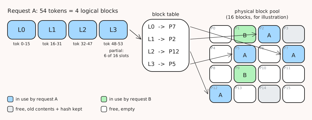
How many blocks exist: startup memory accounting
The block pool’s size is decided once, at startup, by measurement rather than estimation. From determine_available_memory in vllm/v1/worker/gpu_worker.py and request_memory in vllm/v1/worker/utils.py, as of 2026-08-21:
requested        = total_gpu_memory * gpu_memory_utilization   # default 0.92
kv_cache_memory  = requested - weights - peak_activation - non_torch
                   [- cudagraph estimate, if enabled]
num_blocks       = kv_cache_memory / page_size_bytes
Two details matter. gpu_memory_utilization multiplies total device memory, not free memory, so a GPU shared with another process will overcommit unless the setting is lowered (or kv_cache_memory_bytes is set to bypass the calculation entirely). And peak activation memory is measured by running an actual dummy forward pass (profile_run()), not modeled, which is the robust choice given how many configuration knobs affect it.
The per-block byte cost follows the KV formula from the numbers section, restated per block per layer (page_size_bytes, FullAttentionSpec in vllm/v1/kv_cache_interface.py):
For Llama 3 8B at bf16 with block size 16: \(2 \cdot 16 \cdot 8 \cdot 128 \cdot 2 = 64\) KiB per block per layer, times 32 layers = 2 MiB of pool memory per 16-token block, consistent with the 128 KiB/token figure from earlier. At startup vLLM divides the pool by the blocks a maximum-length request would need and logs the result as “Maximum concurrency for … requests” (get_max_concurrency_for_kv_cache_config, vllm/v1/core/kv_cache_utils.py); it’s the first line to read when debugging capacity.
The three layers of the V1 design
Before the data structures, a quick cast of characters, because the rest of this section leans on them. vLLM V1 splits serving across processes (docs/design/arch_overview.md): an API server process handles HTTP and tokenization, and an engine core process runs the serving loop itself. Inside the engine core lives the scheduler: every step, it decides which requests run and how many tokens each gets, and, since KV memory is the resource those decisions hinge on, it also owns all the KV bookkeeping below. The workers (one process driving each GPU) hold the model weights and the physical KV pool, and execute the fused forward pass they are told to run. The division of labor to hold onto: the scheduler decides and does its bookkeeping on the CPU; the workers execute on the GPU; and what crosses between them each step is a small instruction packet, which requests to run, how many tokens each, and which physical block ids to write KV into. The full architecture, why the processes are split this way and what else lives where, gets its own section near the end of the post (The Engine at Runtime); this much is enough for everything here.
With the roles fixed, the memory machinery is three layers:
| Layer | Class / file (as of 2026-08-21) | Job |
|---|---|---|
| Block bookkeeping | KVCacheBlock, BlockPool (vllm/v1/core/block_pool.py) | every block object preallocated at init; tracks ref_cnt and block_hash; free blocks live on an intrusive doubly-linked list |
| Per-request logic | KVCacheManager (vllm/v1/core/kv_cache_manager.py) | get_computed_blocks() (prefix-cache hits), allocate_slots(), free(); called by the scheduler, not the worker |
| GPU-side mapping | block table (vllm/v1/worker/block_table.py) | logical-to-physical indices fed to the attention kernels; append-only in V1 |
One field in that first row needs defining now, because everything below uses it: ref_cnt is a block’s reference count, the number of live requests currently using that block. It exists because blocks can be shared: prefix caching (the next section’s subject) lets several requests point at the same physical block instead of each computing its own copy, and a shared block can only be recycled once nobody points at it, i.e., when its count is back to zero.
Two design choices in that table repay attention. First, every KVCacheBlock is preallocated and the free list is a hand-rolled intrusive doubly-linked list: the scheduler’s hot loop performs allocation and free at very high rates, so this avoids Python object churn, and the intrusive links give O(1) removal from the middle of the free list, which the prefix cache needs when a cache hit pulls a freed block back into service. Second, the scheduler owns all allocation decisions; the worker just receives block ids inside its per-step instructions. Memory is the scarce resource that admission and preemption decisions hinge on, so the policy lives in one place, the engine core, and the worker stays a dumb executor.
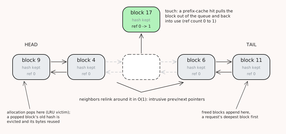
allocate and free, step by step
For a new request, the scheduler first calls get_computed_blocks() to find the longest cached prefix (next section), then allocate_slots():
- Compute how many new blocks are needed; if the pool cannot cover it, return failure (which triggers preemption, covered in the scheduling section).
- “Touch” the cache-hit blocks: increment
ref_cntand remove them from the free queue, so they cannot be evicted while in use. - Pop fresh blocks from the head of the free queue, evicting each popped block’s old cached identity if it had one.
- Register every block that fills completely in the hash map immediately, so that another request in the same batch can already reuse it.
A running request repeats the same flow minus the prefix lookup: fill the last partial block, allocate more as its computed-token count grows. On finish, blocks whose ref_cnt drops to zero are appended to the free queue in reverse order, deepest block first, a small trick with a purpose that will make sense in the prefix-caching section: the block least likely to be reused is placed closest to eviction (docs/design/prefix_caching.md).
The subtle and load-bearing fact: freeing a block does not erase it. A freed block keeps its contents and its hash while sitting in the free queue, and only actually dies when a later allocation pops it and overwrites it. Freed-but-intact blocks are what the prefix cache is made of.
Preemption: free everything, recompute later
Now the failure path. Mid-serving, some running request needs one more block for its next token, and allocate_slots() reports the pool is empty. The engine can’t partially refuse (a request either gets its block or can’t run this step), so one running request must give up its memory so the rest can make progress. The scheduler picks that request, the victim (which one it picks is a policy question, covered in the scheduling section), and Scheduler._preempt_request (vllm/v1/core/sched/scheduler.py) does three things to it:
- All of the victim’s blocks are freed back to the free queue. Per the free semantics above, their contents and hashes stay intact for now; they’ve just become reclaimable by others.
- Its progress counter is zeroed (
num_computed_tokens = 0). The victim keeps its tokens, the prompt and everything it has generated so far live in the request’s CPU-side state; what the engine records is that no KV cache exists for them anymore. - It moves to the front of the waiting queue, first in line to be re-admitted once memory frees up.
Recovery, at re-admission, is recomputation: the victim’s full token sequence (prompt plus its already-generated output) runs through prefill again to rebuild the KV that was thrown away. In the good case even that is cheap: if the victim’s freed blocks are still sitting in the free queue un-overwritten, the prefix-cache lookup finds them and the “recompute” is mostly a cache hit on its own old blocks.
V0 had a second mechanism, swapping a preempted request’s blocks out to CPU memory and back, and V1 deleted it along with the --swap-space flag and its metrics (docs/design/metrics.md): once blocks became shared, deduplicated state under prefix caching, tracking swapped shared blocks was more machinery than it was worth, while free-and-recompute needs nothing beyond what this section already built.
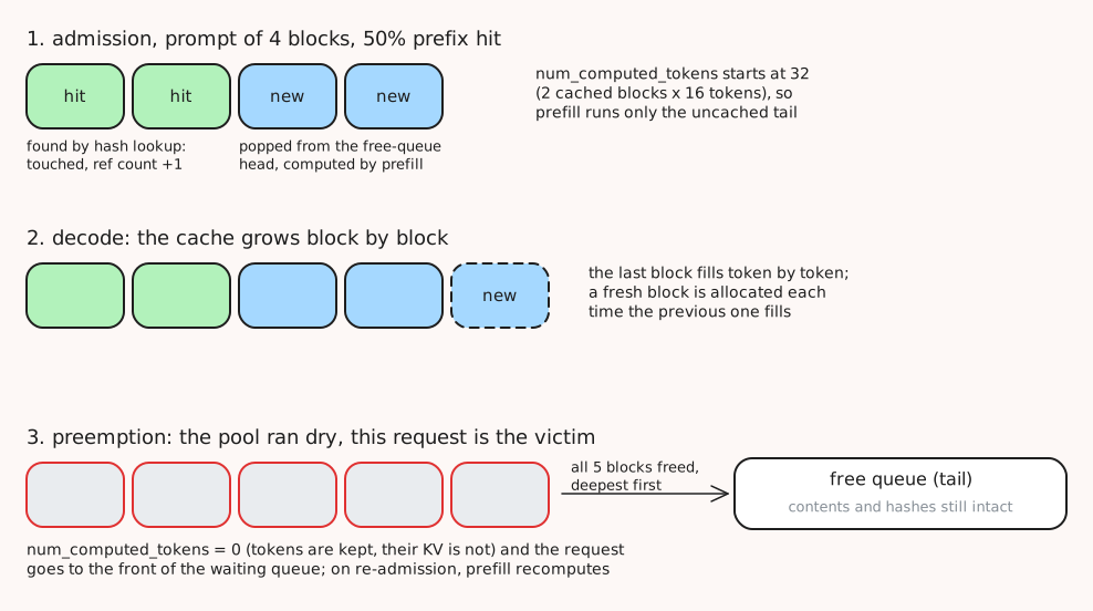
Two closing notes for completeness. Hybrid models (mixing full attention, sliding-window attention, and Mamba state layers) give each layer type its own KV spec and manage them in groups via a hybrid coordinator (vllm/v1/core/kv_cache_coordinator.py, single_type_kv_cache_manager.py, docs/design/hybrid_kv_cache_manager.md). And quantizing the KV cache to fp8 halves page_size_bytes, doubling the block count from the same pool; the per-token-head scales it needs are budgeted inside the page size (vllm/v1/kv_cache_interface.py). More on that in the quantization section.
References
- Efficient Memory Management for Large Language Model Serving with PagedAttention - Kwon et al., SOSP 2023
- vLLM launch blog
- vLLM prefix caching design doc, metrics design doc, hybrid KV cache manager doc
- vLLM source, as of 2026-08-21:
vllm/v1/worker/gpu_worker.py,vllm/v1/worker/utils.py,vllm/v1/kv_cache_interface.py,vllm/v1/core/block_pool.py,vllm/v1/core/kv_cache_manager.py,vllm/v1/core/kv_cache_utils.py,vllm/v1/worker/block_table.py,vllm/v1/core/sched/scheduler.py,vllm/config/cache.py
Prefix Caching
What and why
Prefix caching is the observation that the KV cache is a pure function of the token sequence: same tokens after the same prefix produce the same K and V, always. So when a new request’s prompt shares a prefix with something the engine has already computed, recomputing that prefix’s KV is pure waste; reuse the blocks instead and start prefill at the first novel token. Correctness is exact, the same tokens yield the same KV, so it cannot change model outputs; vLLM’s design doc calls it “almost a free lunch” (docs/design/prefix_caching.md), and it is on by default (enable_prefix_caching: bool = True, vllm/config/cache.py).
The workloads it wins on are the workloads that dominate production: a system prompt shared across every request to a service, multi-turn chat where each turn re-sends the whole conversation so far, and few-shot prompts sharing their examples. One granularity caveat: only full blocks are cached, since a partial block’s KV would depend on tokens still being appended, so hits come in multiples of the block size. The design doc’s example: a 14-token shared prefix with block size 4 hits only 2 blocks, 8 tokens.
The hash chain
The cache key is where the design earns its correctness. Each full block’s hash is
\[\text{hash}(\text{parent\_hash},\; \text{block\_tokens},\; \text{extra\_hashes})\]-
parent_hashchains every block to its entire prefix. This is the crucial bit: a block’s KV depends not just on its own 16 tokens but on everything before them, so the key must encode the whole history. Chaining the parent’s hash does that in constant space, and it means a block hash uniquely identifies “these tokens, after exactly this prefix.” - The block’s exact tokens are included alongside the parent hash to reduce the impact of collisions.
-
extra_hashescarries anything else that changes the KV for identical token ids: the LoRA adapter id, multimodal input hashes, andcache_salt. The multimodal case is worth understanding: two different images tokenize to identical placeholder tokens, so a token-only hash would collide across images; the frontend’s hash of the actual image content is added to every block spanning it. Andcache_saltis a security feature: it’s injected into the first block’s hash, so only requests carrying the same salt can share cache entries. This defends against a real attack, probing response timing to learn whether some other tenant’s prompt is already cached.
The hash algorithm is configurable (--prefix-caching-hash-algo): sha256 is the default since v0.11 (the earlier default was not collision-safe), sha256_cbor gives cross-version reproducibility, and xxhash is fast but non-cryptographic; the docs warn that in multi-tenant settings, constructible collisions can leak private information across requests, so the cheap hash is a real trade and not a free speed win.
Mechanics: the cache that costs nothing
Here’s the elegant part: given the block pool from the previous section, prefix caching needs almost no new machinery. BlockPool keeps one extra map from hash to block (cached_block_hash_to_block, vllm/v1/core/block_pool.py). Lookup (KVCacheManager.get_computed_blocks()) hashes the incoming prompt block by block and walks the chain until the first miss, yielding the longest cached prefix. And the eviction policy falls out of the allocator:
- A freed block keeps its hash and contents in the free queue and remains hittable there.
- Eviction happens only at reallocation: popping a cached block off the free-queue head strips its hash from the map (
_maybe_evict_cached_block). There is no evictor thread, no TTL, no reference-counting sweep; eviction is lazy and embedded in allocation. - LRU ordering comes for free: the free queue is FIFO, freed blocks join at the tail, allocation pops at the head. And the reverse-order freeing from the previous section is the finishing touch: a request’s deepest blocks (encoding its longest, most request-specific prefix, the least likely to be shared) are freed first, landing nearest the eviction head, while shallow blocks (short shared prefixes, like system prompts) survive longest.
- A cache hit “touches” the block, ref_cnt up and off the free queue, so nothing referenced can be evicted.
Two more behaviors complete the picture. Full blocks are registered in the hash map the moment they fill, not when the request finishes, so two same-prefix requests arriving in the same batch still share: the second one hits blocks the first one filled moments earlier. And because V1 block tables are append-only, a decoded block that happens to duplicate an already-cached block is not swapped out for the cached copy; the duplicate simply lives until its request frees it, a small memory cost bought for a simpler runtime (V1 dropped V0’s copy-on-write machinery on the same reasoning: implicit sharing plus recompute-on-preemption covers the cases that matter with near-zero overhead, per the history section of docs/design/metrics.md).
Observability
Hit rate is exported as two counters, vllm:prefix_cache_queries and vllm:prefix_cache_hits (in tokens), so any window’s hit rate is rate(hits)/rate(queries) in PromQL; the periodic log line uses the last 1k queries (docs/design/metrics.md). Programmatic access goes through LLM.get_metrics() (PrefixCacheStats, vllm/v1/metrics/stats.py). Disable with --no-enable-prefix-caching; and when benchmarking with repeated prompts, call reset_prefix_cache() first or the numbers measure the cache, not the model.
One forward pointer: the hash chain names KV content by what it is rather than where it lives, which is exactly what makes KV shareable across machines. The disaggregation section builds on that.
References
- vLLM prefix caching design doc
- vLLM metrics design doc
- vLLM source, as of 2026-08-21:
vllm/v1/core/block_pool.py,vllm/v1/core/kv_cache_manager.py,vllm/v1/metrics/stats.py,vllm/config/cache.py
Scheduling in vLLM V1
There is no prefill phase
The V1 scheduler (Scheduler.schedule() in vllm/v1/core/sched/scheduler.py, as of 2026-08-21) is built on one unifying abstraction, stated in the comment at the top of the function: “There’s no ‘decoding phase’ nor ‘prefill phase’ in the scheduler.” Each request simply carries two counters, num_computed_tokens (how many of its tokens have been through the model) and num_tokens_with_spec (how many it has in total: prompt plus generated plus any speculative tokens), and at each step the scheduler assigns tokens to requests so that the first counter catches up to the second.
It’s worth pausing on how much that one abstraction buys. A fresh prompt is just a request whose computed count is far behind its total: assign it a slice of the gap and you have prefill. Assign it less than the full gap because the budget ran out, and you have chunked prefill, no special case needed. A decoding request is one token behind: assign 1. A prefix-cache hit is a request that starts with num_computed_tokens > 0, so the “prefill” it gets assigned is only the uncached tail. Speculative decoding adds draft tokens to the target count. Five features, one code path, one budget.
The output of a scheduling step is a SchedulerOutput: for each scheduled request, how many tokens to run this step, plus the new KV block ids from allocate_slots(). The worker then executes one fused forward pass for the entire batch, prompt chunks and decodes mixed together.
Budgets and limits
| Knob | Meaning | Defaults (as of 2026-08-21) |
|---|---|---|
max_num_batched_tokens | token budget per step | class default 2048 (vllm/config/scheduler.py); auto-tuned by usage context and GPU in vllm/engine/arg_utils.py: GPUs with 70+ GiB get 8192 (API server) or 16384 (LLM class), smaller GPUs 2048 / 8192 |
max_num_seqs | max concurrently running requests | class default 128; auto-tuned to 1024 (big GPUs) or 256 |
long_prefill_token_threshold | cap on prompt tokens one request may take in one step | 0 = off |
max_model_len | positions cap per request | model-dependent |
Chunking falls out of the budget arithmetic: a request gets \(\min(\text{remaining tokens},\; \text{leftover budget},\; \text{long-prefill threshold if set})\). The other constraint is KV memory: allocate_slots() can fail regardless of the token budget, and that failure is what triggers preemption.
One scheduling step, in order
- Running requests first. Loop over the running list while budget remains: compute each request’s token assignment (usually 1 for a decode, plus any speculative tokens; more if it’s still catching up on its prompt), then try to allocate KV.
- If allocation fails, preempt. Under the default FCFS policy the victim is the most recently added running request (
self.running.pop()); under the priority policy it’s the worst (priority, arrival time) pair, where a larger priority number means less important. Preemption is the full reset from the KV section: all blocks freed, computed count zeroed, victim prepended to the waiting queue to be recomputed later. - Waiting requests next, and only if nothing was preempted this step. Admit while budget remains and the running count is under
max_num_seqs: prefix-cache lookup, then allocation. Requests that are blocked, waiting on remote KV transfer, on structured-output grammar compilation, or on LoRA slot limits (max_lorasper batch), are skipped until unblocked. - Queues are pluggable:
FCFSRequestQueueis a deque;PriorityRequestQueueorders by (priority, arrival time) (vllm/v1/core/sched/request_queue.py;--scheduling-policy fcfs|priority, with a per-requestpriorityfield where lower means more important).
Three consequences of this ordering are the ones to internalize:
- Decodes are effectively prioritized. Running requests are served before waiting ones, and the docs state that chunked-prefill scheduling batches all pending decodes before any prefill (docs/configuration/optimization.md). Running-first protects the ITL of in-flight requests; admission, and therefore TTFT, gets the leftover budget. That’s a deliberate stance on the metrics trade-off from earlier.
- The two ITL knobs. Raising
max_num_batched_tokensbuys throughput and TTFT at the cost of the ITL tail (bigger prefill slices per step);long_prefill_token_thresholdcaps any single request’s slice, protecting the batch at the cost of that request’s TTFT. If p99 ITL spikes correlate with long prompts, these are the two dials. - No admission after a preemption. The guard against admitting when something was just preempted has a simple justification: preemption means memory was insufficient for the current population, so admitting more work in the same step would immediately re-trigger preemption churn.
The other half of the loop
After the model runs, Scheduler.update_from_output() closes the cycle: append the sampled tokens, check token-level stop conditions (EOS, stop token ids, max-token and model-length limits; check_stop in vllm/v1/core/sched/utils.py), free finished requests’ blocks, and carry speculative-decoding bookkeeping (how many draft tokens were accepted) into the next step. Stop strings are the exception: they need detokenized text, so they’re detected in the frontend’s output processor (vllm/v1/engine/output_processor.py), which then aborts the request in the engine core; the runtime section explains why that split exists.
One refinement on top: async scheduling (vllm/v1/core/sched/async_scheduler.py) overlaps the scheduling of step \(N+1\) with the GPU’s execution of step \(N\). The trick is num_output_placeholders: schedule as if the in-flight step’s tokens have already arrived, and reconcile afterwards. This hides the CPU scheduling latency that would otherwise sit between every pair of forward passes.
Seen from a distance, the V1 scheduler is a synthesis of the decade’s two big scheduling ideas: Orca’s iteration-level batching (OSDI ‘22) provides the fluid batch, Sarathi-Serve’s stall-free chunked prefill (arXiv:2403.02310) provides the bounded prefill slices, and the token-budget-with-no-phases formulation is what lets both live in one loop.
References
- Orca - Yu et al., OSDI ‘22
- Sarathi-Serve - Agrawal et al.
- vLLM optimization docs
- vLLM source, as of 2026-08-21:
vllm/v1/core/sched/scheduler.py,vllm/v1/core/sched/request_queue.py,vllm/v1/core/sched/utils.py,vllm/v1/core/sched/async_scheduler.py,vllm/config/scheduler.py,vllm/engine/arg_utils.py
Speculative Decoding
Spending FLOPs that were idle anyway
Recall the decode floor: a decode step reads all 16 GB of weights to produce one token per sequence, using about 16 µs of arithmetic against 4.8 ms of memory time. The compute units are idle 99% of the step. Speculative decoding is the technique that spends that idle compute: let a cheap draft mechanism propose \(k\) tokens, then have the target model verify all \(k\) in a single forward pass, which is possible because given the draft tokens, all \(k\) positions can be computed in parallel, exactly like prefill. A rejection rule then keeps only the longest correct prefix of the draft.
The remarkable property, and the reason the technique is everywhere, is that the output distribution is exactly the target model’s (Leviathan et al., ICML 2023); the paper’s claim is identical outputs, with no change to the distribution. This is a pure latency optimization, not an approximation, in contrast to lossy accelerations like quantization. The catch is scoping: vLLM’s docs recommend it for reducing inter-token latency in memory-bound, medium-to-low QPS regimes (docs/features/speculative_decoding/README.md). At high QPS the batch is already large, decode’s arithmetic intensity approaches the ridge point, the idle FLOPs the technique feeds on disappear, and drafting becomes added load.
The math
With acceptance rate \(\alpha\) (the probability a draft token survives verification) and \(\gamma\) draft tokens per step, the expected number of output tokens per target forward pass is (Leviathan, Eq. 1):
\[\mathbb{E}[\text{tokens per step}] = \frac{1 - \alpha^{\gamma+1}}{1 - \alpha}\]At \(\alpha = 0.8\), \(\gamma = 4\): \((1 - 0.33)/0.2 \approx 3.4\) tokens per weight read instead of 1, a direct multiplier on the decode floor. Note the shape of the formula: gains saturate in \(\gamma\) (the \(\alpha^{\gamma}\) term dies off) while draft cost grows linearly in \(\gamma\), so there’s an optimal draft length that depends on \(\alpha\) and on how expensive drafting is. In practice acceptance also decays with position, because each draft token conditions on previous draft tokens and errors compound; vLLM tracks per-position acceptance counters for exactly this reason (SpecDecodingStats, vllm/v1/spec_decode/metrics.py), and the decay is what caps useful \(\gamma\).
The rejection rule
The exactness guarantee lives in three lines. With \(q\) the draft distribution and \(p\) the target distribution at a given position (vLLM’s implementation, vllm/v1/sample/rejection_sampler.py, states in its docstring that it strictly follows the paper):
- Accept draft token \(x\) with probability \(\min(1,\; p(x)/q(x))\).
- On the first rejection, sample a recovered token from the residual distribution \(\mathrm{norm}(\max(0,\; p - q))\) and stop there.
- If all \(\gamma\) draft tokens are accepted, sample one bonus token from the target’s own distribution at the final position.
Why this is exact: the accepted probability mass at \(x\) is \(q(x)\min(1, p(x)/q(x)) = \min(p(x), q(x))\), and the rejection path’s residual distribution restores precisely the mass \(\max(0, p(x) - q(x))\) that acceptance undercounts; summed, every token’s marginal probability is exactly \(p(x)\). The worst case is 1 token per step (the recovered token), so the scheme is never slower in tokens per step, though it can lose wall-clock time if drafting itself is expensive. One vLLM detail: the bonus token is sampled outside the rejection sampler so the full sampling configuration (top-p, top-k) applies to it.
Where drafts come from
Method (vLLM V1, vllm/v1/spec_decode/) | Draft source | Notes |
|---|---|---|
EAGLE (eagle.py) | a 1-layer head autoregressing on the target’s second-to-top-layer features plus shifted tokens | paper reports 2.7-3.5x latency improvement on LLaMA2-Chat 70B (EAGLE) |
| MTP | the target’s own multi-token-prediction head, if it trained one (DeepSeek-V3 does, tech report) | no separate draft model at all |
| Draft model | a smaller LM from the same tokenizer family | the classic two-model setup |
N-gram (ngram_proposer.py) | prompt lookup: find the most recent match of the current n-gram earlier in the context and copy the tokens that followed it | no model, no training, zero GPU cost |
Suffix decoding (suffix_decoding.py) | a suffix tree over previous outputs, dynamic depth | |
| Medusa, MLP speculator, PARD, custom | see docs/features/speculative_decoding/ |
Configured via --speculative-config '{"method": "eagle", "model": ..., "num_speculative_tokens": k}'. The n-gram proposer deserves a special word: it shines whenever the output copies the input, retrieval-augmented answers quoting their context, summarization, code editing, because the “draft model” is just string matching against text that’s already there. For workloads like that, it’s the first thing to try; a learned draft like EAGLE earns its keep on free-form generation where there’s nothing to copy.
Engine integration
This is where the V1 scheduler’s phaseless design pays off again: speculative decoding required no new scheduling phase. A request’s target count num_tokens_with_spec simply includes the draft tokens, and allocate_slots(..., num_lookahead_tokens) pre-allocates KV blocks for draft tokens that may be rejected. Verification is one forward over context plus \(k\) draft tokens per request, batched together with everything else in the step; the rejection sampler then trims each sequence to its accepted prefix. Rejected tokens waste the KV slots and compute they consumed, their slots are simply reclaimed and overwritten, which is why acceptance-rate monitoring (num_drafts, num_accepted_tokens, and the per-position counters) is the health check that matters for a deployment.
References
- Fast Inference from Transformers via Speculative Decoding - Leviathan et al., ICML 2023
- EAGLE - Li et al.
- DeepSeek-V3 Technical Report
- vLLM speculative decoding docs
- vLLM source, as of 2026-08-21:
vllm/v1/spec_decode/,vllm/v1/sample/rejection_sampler.py,vllm/v1/spec_decode/metrics.py,vllm/v1/core/sched/scheduler.py
Distributed Inference: TP, PP, DP, EP
The numbers section ended on an observation: Llama 3 70B is 140 GB of bf16 weights, and an H100 has 80 GB. Some models simply do not fit on one GPU, and even when they do, the decode floor may be too high; 140 GB over 3.35 TB/s is a 42 ms step, about 24 tokens/s single-stream, if the model fit at all. Parallelism answers both problems, and the four flavors answer them differently.
vLLM’s docs give a clean decision rule worth quoting in spirit (parallelism_scaling.md): if the model fits on one GPU, use no parallelism; too big for one GPU, use tensor parallelism across the GPUs of one node; too big for one node, tensor parallelism within each node times pipeline parallelism across nodes; uneven GPU counts or no NVLink, prefer pipeline over tensor; and if throughput is the problem rather than fit, add whole replicas (data parallelism).
Tensor parallelism: split every matrix
Tensor parallelism (TP) splits each weight matrix across ranks, and vLLM implements Megatron-LM’s scheme (Shoeybi et al.), whose cleverness is in which way each matrix is split. Pair a column-parallel layer (each rank holds a slice of the output dimension) with a row-parallel layer (each rank holds a slice of the input dimension): the column-parallel layer’s sharded output feeds the row-parallel layer’s sharded input directly, with no communication in between, and only the row-parallel layer’s output needs an all-reduce to reassemble the full hidden state.
Both halves of a transformer layer have exactly this two-matmul shape. In vLLM’s Llama implementation (vllm/model_executor/models/llama.py, as of 2026-08-21): attention is QKVParallelLinear (column-parallel, which also splits the heads across ranks) into o_proj as RowParallelLinear; the MLP is MergedColumnParallelLinear (the fused gate/up projection) into down_proj as RowParallelLinear. RowParallelLinear.forward ends with tensor_model_parallel_all_reduce (vllm/model_executor/layers/linear.py), so a decoder layer costs exactly 2 all-reduces per forward pass, each synchronizing the \(d_{model}\) hidden state per token.
Run the numbers for Llama 3 70B: 80 layers times 2 gives 160 all-reduces per token position per step, each carrying a \(8192 \times 2\)-byte = 16 KiB vector per token. That is a torrent of tiny, latency-sensitive messages, the worst possible shape for a network, and it’s why TP effectively requires NVLink and why vLLM ships a family of custom all-reduce kernels rather than relying on NCCL alone (vllm/distributed/device_communicators/: custom_all_reduce.py for NVLink peer-to-peer, plus quick_all_reduce.py, flashinfer_all_reduce.py, symm_mem.py, pynccl.py).
What TP buys is twofold, and the second part is the one people miss: it divides weight memory per rank, and it divides the per-step weight read per rank, which means it is the one parallelism that directly lowers the decode floor. The 70B model’s 42 ms floor becomes roughly 10.5 ms at TP4; the 8B model’s 16 GB read becomes 2 GB per rank at TP8. Pipeline parallelism, next, does neither.
The KV cache shards too, with two traps. KV heads per GPU is \(\max(1,\; H_{kv} / \text{TP})\) (ModelConfig.get_num_kv_heads, vllm/config/model.py), so with Llama 3’s 8 KV heads, TP8 gives 1 head per rank, and TP16 replicates: beyond 8 ranks the per-rank KV footprint stops shrinking. And the code comment adds that MLA (covered in the kernels section) decodes as MQA with a single KV head regardless of TP. Nothing about TP is free, either: as TP grows, there are more and smaller collectives, the per-rank GEMMs get thinner and less efficient, and efficiency per GPU falls.
Pipeline parallelism: split by layers
Pipeline parallelism (PP, --pipeline-parallel-size) cuts the model into contiguous stages of layers, one stage per GPU group. Its communication profile is the mirror image of TP’s: one hidden-state tensor handed point-to-point per microbatch per stage boundary, tiny compared to TP’s per-layer all-reduces, which is why the docs recommend PP across nodes and for machines without fast interconnect, and why it tolerates uneven splits.
The costs are also mirror-imaged. PP adds capacity and throughput but does not improve per-token latency at all: every token still traverses every layer serially, just on different GPUs. And keeping all stages busy requires enough concurrent work in flight; otherwise the pipeline has bubbles. The standard placement for a 2-node, 8-GPU-per-node cluster follows directly: TP8 inside each node (inside the NVLink domain), PP2 across nodes (cheap point-to-point over the network).
Data parallelism: more copies
Data parallelism (DP, --data-parallel-size) runs full replicas of the model with independent request batches. It scales throughput, not model size, and for dense models the replicas are truly independent, DP is just load balancing.
The interesting case is MoE plus MLA models like DeepSeek, where the favored layout is DP for the attention layers combined with TP or expert parallelism for the expert layers (data_parallel_deployment.md). Then DP ranks are no longer independent: the expert layers perform collectives every forward pass, so all ranks’ forward passes must stay aligned, and a rank with no requests of its own must still run empty “dummy” forward passes so its peers’ collectives don’t deadlock; a DP Coordinator process keeps them in lockstep.
Expert parallelism: split the experts
Expert parallelism (EP, --enable-expert-parallel) shards an MoE model’s experts across GPUs, with \(\text{EP} = \text{TP} \times \text{DP}\) (expert_parallel_deployment.md). The router’s decisions turn into all-to-all communication: each token must travel to the GPUs holding its selected experts and back. The backend for that shuffle is selectable (--all2all-backend):
| Backend | Optimized for |
|---|---|
allgather_reducescatter | default; any EP+DP configuration |
deepep_high_throughput | multi-node prefill (grouped GEMM, contiguous layout) |
deepep_low_latency | multi-node decode (CUDA-graph support, masked layout) |
flashinfer_nvlink_one_sided / two_sided | multi-node NVLink domains |
Notice the prefill/decode split reappearing at the communication layer: the two phases want different all-to-all kernels for the same reasons they want different everything else, throughput-shaped bulk transfers for prefill, latency-shaped graph-capturable ones for decode. The two-regime structure from the start of this post runs the whole way down the stack.
Operationally: the executor backend is Python multiprocessing on a single node and Ray for multi-node by default (--distributed-executor-backend mp|ray), and the startup lines worth knowing are “GPU KV cache size: N tokens” and “Maximum concurrency for M tokens per request: X.XXx” (vllm/v1/core/kv_cache_utils.py), both reported per replica.
References
- Megatron-LM - Shoeybi et al.
- vLLM parallelism scaling docs, data parallel deployment, expert parallel deployment
- vLLM source, as of 2026-08-21:
vllm/model_executor/models/llama.py,vllm/model_executor/layers/linear.py,vllm/distributed/device_communicators/,vllm/config/model.py,vllm/v1/core/kv_cache_utils.py
Disaggregated Prefill and KV Transfer
Why split the phases across machines
Everything so far bounded prefill’s interference with decode; disaggregation removes it. Run prefill and decode on separate vLLM instances, on separate GPUs, and ship the KV cache from one to the other. vLLM’s docs give exactly two reasons for doing this (disagg_prefill.md, the feature is marked experimental):
- Tune TTFT and ITL independently. Each instance gets its own parallelism and sizing: give the prefill fleet more TP to cut TTFT without touching the decode fleet’s ITL, or vice versa.
- Control tail ITL by construction. Chunked prefill bounds the interference but leaves a chunk-size knob that the docs concede is hard to set correctly; disaggregation eliminates the interference class, since no decode step ever shares a GPU with a prefill.
And one warning the docs put in bold that deserves repeating: disaggregated prefill does not improve throughput. You pay a KV transfer per request and you run two fleets; the win is SLO attainment, goodput, which is DistServe’s framing of the whole problem (DistServe). The deeper rationale is the roofline again: prefill is compute-bound and decode is memory-bound, so the phases want different quantities of hardware and arguably different hardware generations entirely; Splitwise makes that argument explicitly, noting token generation doesn’t need the compute capability of the newest GPUs (Splitwise). The production proof point is Mooncake, the serving system behind Kimi, a “KVCache-centric disaggregated architecture” with separate prefill and decode clusters and a cache pooled across CPU, DRAM, and SSD; the paper reports up to 525% throughput gains in simulation and 75% more requests served in production under SLOs, plus prediction-based early rejection under overload (Mooncake).
The transfer problem
The catch is physics: the thing being shipped is large. One 8K-token request on Llama 3 70B carries 2.5 GiB of KV; moving that in 100 ms needs 25 GB/s of network. A 32K-token context is 10 GiB (\(32{,}768 \times 320\) KiB), and landing it in under 200 ms needs about 54 GB/s, roughly 430 Gbit/s. Numbers like that are why the transports are RDMA-class (NIXL over UCX, GPUDirect Storage) and why the API is designed to overlap transfer with compute rather than serialize them.
How vLLM implements it
Two or more vLLM instances plus a connector that moves KV from the prefill instance to the decode instance; a kv_role of kv_producer, kv_consumer, or kv_both, with everything under vllm/distributed/kv_transfer/. The connector interface (KVConnectorBase_V1, vllm/distributed/kv_transfer/kv_connector/v1/base.py, as of 2026-08-21) splits cleanly along the engine’s own scheduler/worker line:
- Scheduler-side:
get_num_new_matched_tokens()reports how many of a request’s tokens the remote cache already holds, and it feeds the samenum_computed_tokensmachinery as local prefix caching, so to the scheduler a remote hit looks exactly like a local one.update_state_after_alloc()reacts to allocation, andrequest_finished()decides whether blocks must outlive the request because an async transfer is still reading them; that deferred-free path is what keeps producer memory from leaking while a send is in flight. - Worker-side:
start_load_kv(),wait_for_layer_load(i),save_kv_layer(i),wait_for_save(),get_finished(). The per-layer granularity is the point: the decode instance can start computing layer \(i\) as soon as layer \(i\)’s KV has landed, and the prefill instance can ship layer \(i\) while computing layer \(i+1\), so a multi-GiB transfer overlaps with the forward pass instead of stalling ahead of it.
A request whose KV is still in flight waits in the queue in a blocked state (WAITING_FOR_REMOTE_KVS, vllm/v1/core/sched/scheduler.py) and is skipped by the scheduler until promotable, one of the skip conditions listed back in the scheduling section.
The connector is pluggable, and the zoo (disagg_prefill.md) tells you what people actually deploy:
| Connector | Transport / idea |
|---|---|
NixlConnector | NIXL library, fully async send/recv; backends include UCX and GDS |
LMCacheConnectorV1 | the LMCache caching layer (NIXL underneath); can run a standalone lmcache server shared by instances |
MooncakeConnector | Mooncake’s transfer engine |
MoRIIOConnector | ROCm only |
OffloadingConnector | KV to CPU memory, with its own block size and cpu_bytes_to_use |
FlexKVConnectorV1 | distributed KV store, multi-level cache |
MultiConnector | an ordered list of connectors, e.g. NIXL with a storage fallback |
Configured as --kv-transfer-config '{"kv_connector": "NixlConnector", "kv_role": "kv_both", ...}'.
Offloading is the sibling, not the same thing
KV offloading moves cold blocks down the memory hierarchy of the same serving stack, GPU to CPU RAM to filesystem, instead of evicting them; a prefix-cache miss in GPU memory can then hit in CPU memory and be copied back over PCIe, trading transfer bandwidth for prefill recompute (OffloadingConnector plus vllm/v1/kv_offload/; multi-tier configuration in kv_offloading_usage.md). Disaggregation splits the compute phases across instances; offloading extends the cache of one instance. Mooncake’s pooled datacenter-wide cache is the same offloading idea at cluster scale.
The reason all of this composes so cleanly is the prefix-cache hash chain: a block’s chained hash names “these tokens after exactly this prefix” independent of where the bytes physically live, so a local lookup, a CPU-tier lookup, and a remote-cluster lookup are all the same key computation. That’s what “KV-cache-centric” architectures are built on.
References
- Splitwise - Patel et al., DistServe - Zhong et al., Mooncake - Qin et al.
- vLLM disaggregated prefill docs, KV offloading docs
- vLLM source, as of 2026-08-21:
vllm/distributed/kv_transfer/kv_connector/v1/base.py,vllm/v1/kv_offload/,vllm/v1/core/sched/scheduler.py
Attention Kernels
The remaining three sections descend a level, from the engine to what it launches. They’re deliberately tighter than the sections above: each is a map of the territory with the load-bearing facts, not a full walkthrough.
Why attention gets custom kernels
Every other operation in a transformer’s forward pass is a well-behaved dense op: same shapes for every sequence in the batch, weights as operands, a cuBLAS call away. Attention is the exception, and for a structural reason: its operands are per-request state, the KV cache, with ragged lengths across the batch, and in vLLM those operands are physically scattered across non-contiguous blocks addressed through a block table. No BLAS library can express “multiply against a matrix whose rows live at these 200 scattered addresses, lengths varying per batch element.” Hence dedicated attention kernels, and per-backend “metadata builders” that pack the sequence lengths and block tables into whatever layout each kernel wants.
The performance problem, independent of paging, is memory traffic: naive attention materializes the \(S = QK^\top\) score matrix to HBM, which is \(O(n^2)\) bytes of traffic per head. At long context that traffic, not the FLOPs, is the cost.
FlashAttention, briefly
FlashAttention (Dao et al., 2022) is IO-aware exact attention: tile Q, K, V so the working set stays in on-chip SRAM, and compute the softmax online, tracking a running maximum \(m\) and running denominator \(l\) per row as tiles stream through. When a new tile raises the maximum, all previously accumulated exponentials are too large by a factor of \(\exp(m_{old} - m_{new})\), so the accumulator is rescaled by exactly that factor; this rescaling is what makes single-pass exact softmax possible, and the \(n \times n\) matrix is never written to HBM. In roofline terms, FlashAttention saves bytes, not FLOPs: the arithmetic is unchanged, the \(O(n^2)\) HBM traffic is eliminated, and the op’s arithmetic intensity rises accordingly.
FlashAttention-2 (Dao, 2023) keeps the math and fixes the mapping: fewer non-matmul FLOPs on the hot path, parallelization across the sequence dimension even within a single head, and work split across warps to cut shared-memory traffic, for roughly 2x over FA1 and 50-73% of peak FLOP/s on A100. The sequence-dimension parallelism is the part that matters for inference specifically: a decode or small-batch workload has only batch-times-heads independent work items, too few to fill an H100’s 132 SMs, and splitting along the sequence restores the missing parallelism.
The PagedAttention kernel
The decode kernel that reads a paged cache is worth knowing at the block-diagram level (in-repo walkthrough: docs/design/paged_attention.md, sources in csrc/attention/). For one query token:
- Fetch the request’s block table and loop over the physical blocks it names.
- For each block, dot the query against its keys (the QK stage).
- Run the online-softmax bookkeeping: track the running max, then the exponential sum, normalizing as tiles arrive.
- Weight the values and accumulate (the LV stage), then write the output row.
The contribution of the PagedAttention paper was co-designing this kernel with the block allocator: attention pays one level of indirection through the block table, and in exchange the memory system gets the OS-paging model from earlier. The indirection is cheap precisely because the kernel was built around it.
The backend zoo, and two integration seams
vLLM keeps a registry of attention backends (vllm/v1/attention/backends/registry.py, selection via --attention-backend; each backend’s feature support is validated by validate_configuration() and auto-documented in docs/design/attention_backends.md). The main CUDA ones: flash_attn.py (FlashAttention with paged KV), flashinfer.py, triton_attn.py, and flex_attention.py (PyTorch FlexAttention), plus MLA variants under mla/, Mamba and GDN backends for hybrid models, and ROCm-specific implementations.
Two integration facts foreshadow the runtime section. For torch.compile, the entire attention operation hides behind one custom op, torch.ops.vllm.unified_attention_with_output, so Dynamo sees a single clean graph node instead of tracing ragged, data-dependent internals (docs/design/torch_compile.md). For CUDA graphs, backend capabilities differ and drive the runtime mode: the design doc notes that only FlashAttention 3 supports unified full-graph capture, while others (FlashInfer, FlashMLA, Mamba) support full graphs only for pure decode batches (docs/design/cuda_graphs.md). Attention, in short, is the op that breaks every whole-model optimization, and the engine is architected around walling it off.
MLA in one paragraph
DeepSeek’s Multi-head Latent Attention stores a low-rank latent compression of K and V instead of full per-head KV; the per-head keys and values are re-projected from the latent at compute time. vLLM’s config comment states that MLA during decode becomes MQA with a single KV head (ModelConfig.get_num_kv_heads, vllm/config/model.py), so the cache holds one latent vector per token regardless of TP: a dramatic KV-per-token saving bought with extra projection compute, which is a good trade for a phase whose FLOPs were idle anyway. Dedicated backends live in vllm/v1/attention/backends/mla/.
References
- FlashAttention - Dao et al., FlashAttention-2 - Dao
- PagedAttention - Kwon et al.
- vLLM paged attention kernel walkthrough, attention backends doc, CUDA graphs doc, torch.compile doc
- vLLM source, as of 2026-08-21:
vllm/v1/attention/backends/,csrc/attention/,vllm/config/model.py
Quantization and MoE
Quantization, said via the roofline
Which quantization scheme helps depends entirely on which regime you’re in, and the roofline makes the decision mechanical.
- Weight-only 4-bit (W4A16) cuts weight bytes 4x while computing in 16-bit. That’s a direct attack on memory-bound decode: the 16 GB weight read becomes 4 GB and the decode floor drops proportionally, while the extra dequantization arithmetic is free because the FLOPs were idle. But it does roughly nothing for compute-bound prefill or large-batch throughput, where bytes weren’t the bottleneck.
- W8A8 (FP8 or INT8) quantizes activations too, so the GEMMs themselves run on the 8-bit tensor cores at double the 16-bit rate (Hopper in-depth). That attacks the compute-bound regime as well, and it’s the scheme that helps prefill.
- KV-cache quantization attacks the third byte stream, the one that grows with context and, unlike weights, does not amortize with batch.
The methods behind the checkpoints (vLLM quantization docs):
| Method | Idea | Bits |
|---|---|---|
| GPTQ (Frantar et al., ICLR ‘23) | one-shot post-training weight quantization using approximate second-order information | 3-4 bit weights |
| AWQ (Lin et al., MLSys ‘24 best paper) | activation-aware: protect the ~1% of weight channels with large activations by scaling, no backprop | 4-bit weights |
| FP8 W8A8 | E4M3 weights and activations with per-tensor or per-channel scales; native tensor-core dtype on Hopper | 8 |
| INT8 W8A8, INT4 W4A16, W4A8 | via LLM Compressor |
AWQ’s insight generalizes: quantization error is not uniform, a small set of salient channels (identified by activation magnitude, not weight magnitude) dominates end quality, and protecting just those preserves accuracy at 4-bit. The rule-of-thumb from both papers’ results: weight-only 4-bit is near-lossless at 7B+ scale, while activation quantization is the hard part (outlier channels), which is why W8A8 needs calibration and scales while W4A16 barely does. On the kernel side, quantized weights need dequantization fused inside the GEMM, a dedicated kernel family: vLLM’s hardware table lists Marlin kernels for GPTQ/AWQ/FP8/FP4 on Ampere and newer, with sources under csrc/quantization/. vLLM ingests checkpoints from AutoAWQ, BitsAndBytes, GPTQModel, LLM Compressor, NVIDIA ModelOpt, TorchAO, Quark, and GGUF, plus online quantization.
The KV-cache variant (quantized_kvcache.md): kv_cache_dtype="fp8" (E4M3 on CUDA and ROCm, E5M2 optional on CUDA), with per-tensor or per-head scales. One default to know before flipping it on: calibration is off by default and all scales are 1.0 (calculate_kv_scales=False), which assumes the K/V values fit E4M3’s range as-is; real outliers will clip or lose precision silently. The alternatives are dynamic scale computation (calculate_kv_scales=True) or a checkpoint with calibrated scales. The capacity payoff is exactly the block-pool formula from earlier with \(b\) going from 2 to 1: half the page size, double the blocks, roughly double the maximum concurrency or context.
MoE essentials
A Mixture-of-Experts layer replaces the dense FFN with \(E\) expert FFNs plus a router that sends each token to its top-\(k\) experts. Compute per token stays roughly \(k\) experts’ worth while parameter count scales with \(E\); DeepSeek-V3 is 671B total parameters with 37B activated per token (tech report). The catch for serving: all 671B must be resident, because any token may route to any expert. MoE thus moves the bottleneck from FLOPs to memory capacity and communication, which is why it’s the architecture that forces EP and wide NVLink domains.
Two problems define the MoE serving stack. The kernel problem: each token multiplies a different weight matrix, so a plain GEMM is impossible; the fused MoE kernels (vllm/model_executor/layers/fused_moe/, Triton) sort and group tokens by expert, run grouped or batched GEMMs, apply the activation, and scatter results back weighted by router probabilities, all fused to avoid materializing the intermediate shuffles. The placement problem: routing is skewed, so some experts’ GPUs saturate while others idle, and the step takes the max over GPUs; EPLB, the expert parallelism load balancer (vllm/distributed/eplb/), re-places and replicates experts against the observed routing load to flatten that max. Together with the phase-specialized all-to-all backends from the distributed section, that’s the MoE serving picture.
References
- GPTQ - Frantar et al., AWQ - Lin et al.
- vLLM quantization docs, quantized KV cache
- DeepSeek-V3 Technical Report, NVIDIA Hopper architecture in-depth
- vLLM source, as of 2026-08-21:
csrc/quantization/,vllm/model_executor/layers/fused_moe/,vllm/distributed/eplb/
The Engine at Runtime
Two processes
vLLM V1 splits the engine across two process roles (arch_overview.md, multiprocessing.md): the API server process handles HTTP, input processing (tokenization, multimodal media), and streaming results back; the engine core process runs the scheduler, manages the KV cache, coordinates the GPU workers, and runs a busy loop. They communicate over ZMQ sockets, and under data parallelism the API servers scale out to match, every API server connected to every engine core.
The design principle behind the split is stated in the metrics doc and explains half the architecture: the engine core is the inner loop where performance is critical, so anything that can live in the frontend, detokenization, stop-string scanning, metrics assembly, does, where it overlaps with GPU execution instead of adding to it. Time spent on the CPU between forward passes is added ITL for every running request; time spent in the frontend is free. That’s why stop strings are detected in the frontend’s output processor (as noted in the scheduling section): they need detokenized text, and detokenization was banished from the hot loop.
One request’s life, end to end: HTTP in, tokenize in the frontend, cross ZMQ, wait QUEUED in the engine core, get tokens and KV blocks assigned by the scheduler (SCHEDULED), run in the fused forward pass, sampled token crosses back per iteration in EngineCoreOutputs, frontend detokenizes, checks stop strings, streams the delta out. On the GPU side, the model runner (vllm/v1/worker/gpu_model_runner.py, as of 2026-08-21) keeps a persistent input batch (gpu_input_batch.py) that is updated incrementally as requests enter and leave rather than rebuilt per step, builds the per-backend attention metadata, launches the compiled-and-graphed model, and samples.
torch.compile
vLLM compiles the model with a structure dictated by attention (torch_compile.md). Dynamo captures the forward as a full graph, with attention appearing as the opaque unified_attention_with_output custom op from the kernels section. The graph is then split at the attention ops into piecewise submodules; for a Llama-style model that yields three unique subgraphs (before the first attention, the repeated middle between attentions, after the last), and the repeated middle compiles once and is reused. Compiled artifacts are cached on disk keyed by everything that was traced, model code, the vLLM files involved, and the relevant config, so any change to any of them is a cache miss and a recompile (~/.cache/vllm/torch_compile_cache/...). Batch and sequence dimensions are symbolic, with guard-dropping modes (backed_size_oblivious, unbacked) controlling the recompile-versus-guard-risk trade.
CUDA graphs
Here’s where the kernel-launch overhead from the numbers discussion comes due. A decode step launches hundreds of small kernels for a few milliseconds of total GPU work; at microseconds of CPU launch overhead each, the launches themselves become a tax on exactly the step the decode floor already made expensive. CUDA graphs fix it by capturing the whole kernel sequence once and replaying it with a single launch.
The complication, once again, is attention. vLLM’s answer (cuda_graphs.md) is piecewise capture: the token-wise subgraphs between attentions (which is what the torch.compile split above produced) are captured as CUDA graphs, and attention runs eager in the gaps, since its ragged, paged, data-dependent access is, in the doc’s words, non-trivial to make cudagraph-compatible. A supporting detail with a purpose: the attention op takes its output tensor as an input, so all memory allocation stays inside the graphed pieces and pointers remain stable across replays.
The runtime modes (cudagraph_mode): NONE, PIECEWISE, FULL, FULL_DECODE_ONLY (useful for the decode fleet of a disaggregated setup), and the default FULL_AND_PIECEWISE: full graphs for uniform decode batches, piecewise for everything else. A CudagraphDispatcher (vllm/v1/cudagraph_dispatcher.py) picks the mode per batch, preferring FULL over PIECEWISE over NONE, and pads each batch up to the nearest pre-captured size (cudagraph_capture_sizes), so the padding waste is bounded by the gap between consecutive capture sizes. Backend capability drives automatic downgrades (the FlashAttention-3-only full-capture caveat from the kernels section), and the doc is candid about the cost of the default: most performant, but the most memory and the longest capture time at startup.
Sampling
The last stop in the loop (Sampler.forward, vllm/v1/sample/sampler.py): apply logits processors and penalties, apply temperature, then greedy or random sampling with top-k/top-p, gather logprobs if requested, and merge speculative-decoding outputs. Greedy has a shortcut path, and temperature 0 maps to it. Structured output (JSON schemas, grammars) costs almost nothing at this point: the scheduler ships a grammar bitmask computed off the hot path (Scheduler.get_grammar_bitmask; requests wait in a blocked state during grammar compilation, one of the scheduling section’s skip conditions), and the sampler applies the mask to the logits before sampling, one masked-fill per step.
References
- vLLM architecture overview, multiprocessing doc
- vLLM CUDA graphs doc, torch.compile doc, metrics design doc
- vLLM source, as of 2026-08-21:
vllm/v1/worker/gpu_model_runner.py,vllm/v1/worker/gpu_input_batch.py,vllm/v1/cudagraph_dispatcher.py,vllm/v1/sample/sampler.py,vllm/v1/core/sched/scheduler.py
Test Yourself
Everything above, as questions. Try answering each from memory before reading its answer; every answer traces back to a section of this post, and the sources are in those sections’ references. If a group feels shaky, that’s the section to reread.
The numbers
1. H100 SXM memory bandwidth and dense BF16 TFLOPS? Ridge point? 3.35 TB/s and ~1000 TFLOPS dense (1,979 “with sparsity”). Ridge \(\approx 10^{15}/3.35\times10^{12} \approx 300\) FLOP/byte.
2. KV bytes per token for Llama 3 70B in bf16? In fp8? \(2 \cdot 80 \cdot 8 \cdot 128 \cdot 2 = 320\) KiB/token in bf16; halve the bytes-per-element for fp8: 160 KiB.
3. Why is the marketing TFLOPS number double the usable one? It assumes 2:4 structured sparsity, which doubles the rate. Dense workloads, LLM inference included, get the dense number, half of it.
4. Minimum decode step time for a 70B bf16 model on one H100, and the implication? 140 GB / 3.35 TB/s \(\approx\) 42 ms, so ~24 tok/s single-stream, and the model doesn’t even fit in 80 GB. TP splits the weight read across ranks, cutting both memory per rank and the floor (TP4: ~10.5 ms).
5. At what batch size does decode stop being weight-bandwidth-bound on H100, roughly? Around the ridge point, ~300 sequences, since decode’s arithmetic intensity is roughly the batch size. KV reads scale with batch times context and don’t amortize, pushing the real crossover higher.
The problem and metrics
1. Why is decode memory-bound if it does the same \(2N\) FLOPs per token as prefill? Same FLOPs, different amortization of bytes: prefill reads the weights once for \(P\) tokens (intensity \(\approx P\), above the ridge); decode reads them for 1 token per sequence (intensity \(\approx B\)). Below the ridge, bytes dominate and the FLOPs are irrelevant.
2. ITL vs TPOT: definitions, and which exposes a preemption? ITL is the gap between consecutive tokens, one sample per step; TPOT is \((\text{E2EL} - \text{TTFT})/(n-1)\), a per-request mean. A preemption is one huge ITL sample that TPOT smears into the average, so ITL p99 exposes it.
3. Why does a long prompt hurt other requests’ latency, and what bounds it? Its prefill tokens ride in the same forward pass as everyone’s decodes and stretch the step, which every co-batched request inherits as ITL. Chunked prefill bounds the per-step chunk via the token budget, trading that request’s TTFT.
4. A vendor claims 5000 tok/s versus another’s 3000. What do you ask? Batch size and the latency distribution; the SLOs (goodput), prompt/output length mix, arrival pattern, and client- versus engine-side measurement. Throughput without a latency constraint is purchasable with batch size and not comparable.
5. What does client-measured TTFT include that engine-measured TTFT does not? Network, HTTP, and client-side stream handling; engine TTFT starts at frontend arrival (tokenization). The delta isolates everything outside the engine.
6. Why does throughput rise roughly linearly with batch size, then flatten? What sets the knee? Each added sequence reuses the same weight read while memory-bound, so tokens/s scales almost linearly; the knee is where arithmetic intensity reaches the ridge point, bent earlier by growing KV traffic.
7. Static vs continuous batching: what specifically is wasted in static? Finished requests’ slots idle until the whole batch drains, and arrivals wait for the drain. Continuous batching re-forms the batch every step.
8. Is a preemption counted in vLLM’s decode-time histogram or reset, and why does that make sense? Counted in: the decode interval spans first to last token including the gap, and only the first SCHEDULED sets the timestamp. The user experienced the gap, so SLO-facing histograms should include it.
KV cache and PagedAttention
1. Name the three kinds of waste in contiguous per-request KV allocation and which ones paging eliminates. Over-reservation for an unknown output length, internal fragmentation in the tail, external fragmentation between regions. Paging eliminates reservation (allocate per block on demand) and external entirely; internal remains, bounded per sequence.
2. What bounds internal fragmentation per sequence, numerically? At most \(\text{block\_size} - 1 = 15\) wasted token slots, in the last partial block; under 4% overall per the launch blog.
3. Walk through admission with a 50% prefix-cache hit. get_computed_blocks hash-walks the prompt and returns the cached prefix blocks; allocate_slots touches them (ref count up, off the free queue), pops fresh blocks from the free-queue head for the rest (evicting their old identities), and registers full blocks in the hash map. num_computed_tokens starts at the hit length, so prefill computes only the tail.
4. Why preallocate every KVCacheBlock and hand-roll an intrusive linked list? The scheduler’s hot loop allocates and frees at very high rates; preallocation avoids Python object churn, and intrusive links give O(1) removal from the middle of the free list when a cache hit touches a freed block.
5. How does vLLM size the block pool at startup, and what does gpu_memory_utilization = 0.92 multiply? Total device memory times 0.92, minus measured weights, peak activation (an actual dummy forward), and non-torch overhead, divided by the per-block page size. It multiplies total memory, not free memory.
6. Who calls allocate_slots, and why does that placement matter? The scheduler, in the engine core. Memory is the scarce resource that admission and preemption hinge on, so allocation lives where those decisions are made; workers just receive block ids.
7. What happens to a preempted request’s state in V1, and how is that different from V0? All blocks freed, num_computed_tokens reset to 0, prepended to waiting; recovery is recompute, possibly accelerated by prefix hits. V0 could swap blocks to CPU; V1 dropped swap because shared blocks plus recompute is simpler.
8. A block is “freed”. Is its content gone? No: content and hash survive in the free queue and remain hittable. The block dies only when a later allocation pops it and evicts its hash.
Prefix caching
1. What three components go into a block hash, and why each? The parent hash (chains to the entire prefix), the block’s exact tokens (collision resistance), and extra hashes (LoRA id, multimodal hashes, cache_salt) for anything else that changes the KV.
2. Why cache full blocks only? A partial block’s KV depends on tokens still being appended, and the hash chain needs complete units. Consequence: hits come in multiples of the block size.
3. How does eviction work with no evictor thread or TTL? Freed-but-cached blocks queue FIFO; allocation pops the head, and popping a cached block strips its hash. Eviction is lazy, embedded in allocation, and LRU by construction.
4. Why are a request’s blocks freed tail-first? The deepest block encodes the longest, most request-specific prefix, least likely to be reused; freeing it first puts it nearest the eviction head.
5. Two requests with the same prompt arrive in the same batch. Does the second hit the cache? Yes, once the shared blocks fill: full blocks are hash-registered at fill time, not at request completion.
6. Why does an image need an extra hash when its placeholder tokens are already in the block? Different images tokenize to identical placeholders, so token-only hashes would collide across images; the frontend’s content hash disambiguates.
7. What attack does cache_salt mitigate, and how? Timing probes: an adversary measures latency to learn whether another tenant’s prompt is cached. Salting the first block’s hash partitions the cache by trust group.
8. Why can a cheap hash algorithm be a privacy problem in multi-tenant serving? Constructible collisions could let an attacker poison or read KV across requests; a non-cryptographic hash makes collisions easier, hence the docs’ warning.
Scheduling
1. “There is no prefill phase in the V1 scheduler.” What replaced it? Every request just has num_computed_tokens catching up to num_tokens_with_spec; assigning “how many tokens this step” subsumes prefill, chunking, decode, prefix hits, and speculative decoding in one code path under one token budget.
2. Who gets preempted under FCFS? Under priority? What happens to the victim? FCFS: the most recently added running request. Priority: the worst (priority, arrival time) pair. The victim loses all blocks, resets its computed count, and goes to the head of the waiting queue; its ITL spikes and its decode interval absorbs the gap.
3. Why schedule running requests before waiting ones? Running-first protects in-flight ITL; admission (prefills) gets the leftover budget, which is what keeps decode steps flat under chunked prefill. TTFT is protected only by leftover budget and queue policy.
4. p99 ITL spikes correlate with long prompts. Which two knobs, and their trade-offs? max_num_batched_tokens (bigger buys throughput and TTFT, worse ITL tail) and long_prefill_token_threshold (caps one request’s slice per step, worse TTFT for that request).
5. Why is admission halted in a step that preempted someone? Preemption means memory was insufficient for the current set; admitting more would immediately re-trigger preemption churn.
6. Where does prefix caching plug into scheduling? At admission: get_computed_blocks sets num_computed_tokens to the cached-prefix length, so the scheduler assigns only the uncached tail. A full-prompt hit still schedules at least one token to produce output.
7. What does async scheduling overlap, and via what trick? Scheduling of step \(N+1\) with GPU execution of step \(N\), using num_output_placeholders to schedule as if in-flight tokens had already arrived.
8. What limits concurrency besides max_num_seqs? KV block availability (allocate_slots can fail far earlier), plus the multimodal encoder budget, LoRA slot limits, and grammar-compilation readiness for structured output.
Speculative decoding
1. State the acceptance rule and argue the output distribution is unchanged. Accept draft token \(x \sim q\) with probability \(\min(1, p(x)/q(x))\); on rejection, sample from \(\mathrm{norm}(\max(0, p - q))\). Accepted mass at \(x\) is \(\min(p(x), q(x))\), and the recovery distribution restores exactly the shortfall, so the marginal is exactly \(p\).
2. Expected tokens per step for \(\alpha = 0.7\), \(\gamma = 3\)? \((1 - 0.7^4)/(1 - 0.7) = 0.7599/0.3 \approx 2.53\).
3. Why does speculative decoding help precisely because decode is memory-bound? The weights are read anyway; verifying \(k\) extra tokens rides along on idle FLOPs. More tokens per weight read is a direct attack on the decode floor.
4. Why does per-position acceptance decay, and what does that imply for \(\gamma\)? Each draft position conditions on previous draft tokens, so errors compound. Past the point where \(\alpha^\gamma\) is small, extra draft length adds cost but almost no accepted tokens.
5. When would n-gram beat EAGLE despite having no model? When the output copies the context: RAG quoting, summarization, code edits. String lookup drafts those spans at zero GPU cost with no second model to host.
6. What happens to the KV blocks of rejected draft tokens? They were pre-allocated via num_lookahead_tokens; the slots are reclaimed and overwritten. The waste is the drafted-and-verified compute.
7. Why does the gain shrink at high QPS? Large batches push decode’s arithmetic intensity toward the ridge; the idle FLOPs disappear and drafting becomes added load, which is why the docs scope the feature to medium-to-low QPS.
8. What is the bonus token, and why is it sampled outside the rejection sampler? The extra token appended when all \(\gamma\) drafts are accepted, sampled from the target; it’s sampled outside so the full sampling configuration (top-p/top-k) applies.
Distributed inference
1. Why pair a column-parallel with a row-parallel layer, and how many all-reduces per layer result? The column-parallel output stays sharded and feeds the row-parallel input with no communication; only the row-parallel output needs an all-reduce. Attention plus MLP gives 2 all-reduces per layer.
2. What per-token communication does TP8 decode on Llama 3 70B incur, and why NVLink? \(2 \times 80 = 160\) all-reduces per token, each on a 16 KiB hidden vector: small, frequent, latency-bound messages, exactly what NVLink and custom all-reduce kernels exist for.
3. TP vs PP: which reduces per-token latency, and why? TP: each rank reads \(1/\text{TP}\) of the weights per step, so the memory-bound floor drops. PP doesn’t: every token still crosses all layers serially; PP adds capacity and throughput only.
4. Where do TP and PP go in a 2-node, 8-GPU-per-node cluster? TP8 inside each node (NVLink domain), PP2 across nodes (one cheap point-to-point hidden-state transfer per microbatch per boundary).
5. Why do DP ranks of an MoE model need dummy forward passes? Expert layers run collectives every forward; a rank with no work must still participate or its peers deadlock, so idle ranks run empty passes, coordinated by the DP Coordinator.
6. Why different all-to-all backends for prefill and decode? Prefill wants throughput (grouped GEMM, contiguous layouts: deepep_high_throughput); decode wants latency and CUDA-graph compatibility (deepep_low_latency, masked layout).
7. What gets worse as TP grows? More and smaller collectives, thinner and less efficient per-rank GEMMs, and beyond num_kv_heads the KV cache stops sharding. Efficiency per GPU falls.
8. How does TP change each rank’s KV footprint? KV heads per rank is \(\max(1, H_{kv}/\text{TP})\): Llama 3’s 8 heads shard down to 1 at TP8, and TP16 replicates with no further saving. MLA decodes as MQA, 1 latent head regardless.
Disaggregation and KV transfer
1. The two documented reasons for disaggregated prefill, and the one thing it does not improve? Independent TTFT/ITL tuning per fleet, and tail-ITL control by removing prefill interference. Explicitly not improved: throughput.
2. Chunked prefill and disaggregation both control tail ITL. When is disaggregation the better answer? Chunked prefill needs a well-chosen chunk size, which the docs concede is hard; disaggregation removes the interference class at the cost of a KV transfer and a second fleet. Strict ITL SLOs at scale favor it.
3. Sketch a request’s path through a prefill/decode split. The prefill instance computes the full prompt, saving KV per layer through the connector; the decode instance’s scheduler learns the remote cache holds the prefix via get_num_new_matched_tokens() (the same num_computed_tokens slot as prefix caching), the request waits in WAITING_FOR_REMOTE_KVS until loaded, then decodes normally.
4. Why does the connector API have per-layer load and save hooks? So transfer overlaps compute layer by layer instead of serializing a multi-GiB blob before any work starts.
5. Estimate the bandwidth to move a 32K-token Llama 3 70B context in under 200 ms. \(32\text{K} \times 320\) KiB = 10 GiB \(\approx\) 10.7 GB; over 200 ms that’s ~54 GB/s \(\approx\) 430 Gbit/s: RDMA-NIC territory, hence NIXL, UCX, and GDS.
6. KV offloading versus disaggregation? Offloading moves cold KV down the same stack’s memory hierarchy (CPU RAM, disk) to extend cache capacity; disaggregation splits the compute phases across instances. Same connector API, different job.
7. What does Mooncake add beyond a prefill/decode split? A KV-cache-centric global scheduler over cache pooled across CPU, DRAM, and SSD cluster-wide, plus overload handling with prediction-based early rejection.
8. Why is the block hash the natural addressing scheme for remote KV? The chained hash names “these tokens after exactly this prefix” independent of where the bytes live, so local and remote lookup are the same key computation.
GPU and roofline
1. Define occupancy and the mechanism by which it hides latency. Active warps per SM over the maximum. The SM issues from any ready warp, so one warp’s memory stall is covered by another’s work.
2. Compute the H100 ridge point for dense BF16 and place batch-64 decode on the roofline. \(\approx 10^{15} / 3.35 \times 10^{12} \approx 300\) FLOP/byte. Batch-64 decode has intensity \(\approx 64\): memory-bound, attaining roughly \(64/300 \approx 21\%\) of peak.
3. Why does fusing a norm into a neighboring op help while fusing two GEMMs usually does not? A norm has \(O(1)\) intensity; fused, it rides on bytes already moving and removes a full read-write pass. GEMMs are each compute-bound with tiled reuse; fusing saves little traffic and breaks their optimal tilings.
4. TMA and thread block clusters, one sentence each. TMA: a per-SM DMA engine for asynchronous bulk global-to-shared transfers. Clusters: co-scheduled blocks across SMs that can access each other’s shared memory.
5. Why does FP8 shift both the roof and the kernel’s position? It doubles peak FLOP/s (roof up) and halves bytes per element (the same computation’s intensity up); both shifts push toward compute-bound.
6. A kernel sits at 40% of peak FLOP/s. What single question decides the optimization direction? Is its arithmetic intensity above or below the ridge point? Below: cut bytes (fusion, dtype, layout). Above: raise math throughput (tensor cores, occupancy, scheduling).
Attention kernels
1. What does FlashAttention save, FLOPs or bytes? Bytes. The attention is exact, FLOPs unchanged; tiling keeps the \(n \times n\) scores in SRAM, eliminating \(O(n^2)\) HBM traffic and lifting the op’s arithmetic intensity.
2. Walk through online softmax: which two scalars, and why rescale? A running max \(m\) (numerical stability) and running denominator \(l\). A new tile can raise \(m\), making all previously accumulated exponentials too large by \(\exp(m_{old} - m_{new})\); rescaling by that factor keeps the single-pass accumulation exact.
3. What did FA2 change, and why does within-head parallelism matter for inference? Fewer non-matmul FLOPs, parallelism across sequence blocks within a head, warp-level partitioning to cut shared-memory traffic; ~2x FA1. Decode and small-batch have too few batch-times-heads work items to fill the SMs, so sequence-dimension parallelism is what keeps them busy.
4. How does the PagedAttention kernel find its KV? Through the request’s block table: logical position to physical block id to contents, looping over the table’s blocks doing QK, online softmax, then value accumulation.
5. Why does attention break CUDA-graph capture and torch.compile tracing, and how does vLLM wall it off? Ragged lengths, block tables, and paged gathers are data-dependent control that capture and tracing can’t specialize. torch.compile hides it behind the unified_attention_with_output custom op; CUDA graphs exclude it via piecewise capture (or require a backend like FlashAttention 3 for full capture).
6. Why does MLA decode like MQA, and what’s the KV win? It caches one shared latent projection instead of per-head KV (get_num_kv_heads returns 1), so KV per token shrinks to the latent size, paid for with extra projection compute.
Quantization and MoE
1. W4A16 vs W8A8: which regime does each attack? W4A16 cuts weight bytes: memory-bound decode. Compute still runs 16-bit, so compute-bound prefill sees little; W8A8 runs the GEMMs on 8-bit tensor cores, doubling math throughput there.
2. What makes AWQ “activation-aware”, and why does 1% of channels matter? It scales weight channels by activation magnitude: the ~1% of channels with large activations dominate quantization error, and protecting them preserves accuracy at 4-bit with no backprop.
3. vLLM’s default fp8 KV scales are 1.0. Why is that risky? Unit scales assume values fit E4M3’s range; real outliers clip or lose precision silently. Alternatives: calculate_kv_scales=True or a checkpoint with calibrated scales.
4. What does fp8 KV do to max concurrency, via which formula? Bytes per element drops 2 to 1 in the KV-per-token formula, halving page_size_bytes, doubling num_blocks, and roughly doubling max concurrency.
5. Why does a 671B-parameter MoE with 37B active still need massive memory, and which parallelism answers it? Any token may route to any expert, so all parameters must be resident. Expert parallelism shards the experts, paying with all-to-all routing.
6. What does the fused MoE kernel fuse, and why is a plain GEMM impossible? Routing bookkeeping with the expert GEMMs: sort and group tokens by expert, run grouped GEMMs, scatter back weighted by router probabilities. A plain GEMM is impossible because each token multiplies a different weight matrix.
7. What is EPLB balancing, and why does routing skew hurt? Expert load across GPUs: skewed routing saturates some GPUs while others idle, and the step takes the max over GPUs. EPLB re-places or replicates experts to flatten it.
Engine runtime
1. Why two processes, and what crosses the ZMQ boundary? To isolate the latency-critical scheduler-plus-GPU loop from Python-heavy HTTP and tokenization. In: tokenized requests. Out: EngineCoreOutputs (token ids, events, stats) per iteration.
2. Why does detokenization live in the frontend? Anything between forward passes is added ITL for every running request; frontend work overlaps with GPU execution instead.
3. What are piecewise CUDA graphs, and why is attention excluded? The token-wise subgraphs between attentions are captured and replayed; attention runs eager because its ragged, paged, data-dependent access doesn’t fit capture.
4. Why does the attention op take its output tensor as an input? So the graphed pieces own all memory allocation: eager attention writes into a graph-managed buffer, keeping pointers stable across replays.
5. What triggers a torch.compile cache miss? Any change to traced inputs: model source, inlined vLLM code, or relevant config; the cache directory is keyed on all of it.
6. What does FULL_AND_PIECEWISE do for a mixed batch versus a uniform decode batch? Mixed: dispatched to piecewise graphs, attention eager. Uniform decode: dispatched to the full graph captured for that size. The dispatcher picks per step, preferring FULL, then PIECEWISE, then NONE.
7. Why pad batches under CUDA graphs, and what bounds the waste? Graphs replay fixed shapes, so batches pad up to the nearest captured size; waste is bounded by the gap between consecutive capture sizes.
8. Where is structured output enforced, and what does it cost per step? The scheduler ships a grammar bitmask; the sampler masks invalid logits before sampling. Cost is one mask application per step, with grammar compilation off the hot path.
Wrapping up
If one thing from this post survives, let it be the accounting habit: before reasoning about any part of the serving stack, ask what the bytes are doing. Prefill and decode split because of how they amortize the weight read. The decode floor is a division of two numbers you now know. Batching, speculative decoding, tensor parallelism, and weight quantization are the four distinct attacks on that floor: more tokens per read, more tokens per read again, the read split across GPUs, and a smaller read. The KV cache is the state that makes serving a systems problem; paging packs it, prefix caching deduplicates it, the hash chain names it, and offloading and disaggregation move it. And the scheduler is where all of it meets the metrics: every knob in it is a position on the TTFT-versus-ITL trade, not a way out of it.
The other thing worth keeping is the pattern of the vLLM V1 design itself: one token-budget abstraction where there could have been five phases, eviction embedded in allocation where there could have been an evictor thread, recompute where there could have been swap machinery, measurement where there could have been estimates. Every one of those choices trades a little theoretical capability for a lot of simplicity in the hot loop, and the hot loop is where an inference engine lives or dies.
If you find a mistake anywhere in here, please let me know and I’ll fix it.