DeepSeek's Attention and KV Cache - From MLA to CSA2, From First Principles
Hello all. This post is about one number and how it was driven down. The number is the size of the KV cache a DeepSeek model has to keep in GPU memory for every token of context, and the DeepSeek-V4.1-Flash model card puts its history in a single chart: 389,120 bytes per token for the first DeepSeek LLM in 2023, 48,068 for V3.2 at the end of 2025, 3,514 for V4-Flash in April 2026, and 890 for V4.1-Flash this month. That is a 437-fold reduction in under three years, and every step of it is an architectural idea with a name: Multi-head Latent Attention, sliding windows, the lightning indexer, compressed sparse attention, cross-layer reuse, the causal encoder-decoder, FP4 caches, bounded replay.
I needed to understand all of them at once to reason about serving the newest model, and found that each one is only explicable as the fix for the cost the previous one left behind. So this post walks the lineage in order. Each mechanism gets the same treatment: the cost it attacks, what it does with actual tensor shapes, what it stores per token in bytes, and a diagram. Two short numpy checks are included where a claim is easy to test on a laptop. By the end you can rebuild the 890 from parts, and the chart above stops being a marketing figure and becomes arithmetic.
The plan:
- The cost being cut: KV bytes per token as a product of four levers, and the numbers for four generations
- DeepSeek-V2: Multi-head Latent Attention, the decoupled RoPE key, and weight absorption
- Sliding window attention: bounded caches, stacked receptive fields, and how far they really reach
- DeepSeek-V3.2: sparse attention with a learned indexer
- A precision primer: E4M3, block scales, E2M1, MXFP4, and NVFP4
- DeepSeek-V4: compress the sequence, then sparsify, with a window in every layer
- DeepSeek-V4.1: reuse across layers, project across halves, and store in four bits
- The arithmetic, rebuilt from parts
- Takeaways, and a question bank
I’m assuming the LLM inference systems post as background: what a KV cache is and why decode is bound by bytes rather than FLOPs, paged KV, and the one-paragraph description of MLA there, which this post expands into a section. The companion briefing on serving V4.1-Flash with vLLM covers what these mechanisms cost at deployment; this post is the “why” underneath it. Every number is from a linked paper, model card, or repository, and where I derive something the computation is shown. Config values come from each model’s config.json on Hugging Face, checked on 2026-09-12.
Let’s get started.
The Cost Being Cut
Four levers
A decoder-only transformer must keep, for every token it has seen, whatever later tokens will attend to. In a standard multi-head attention layer that is a key vector and a value vector per head, so the cache per token is
\[\text{bytes per token} = \underbrace{L}_{\text{layers}} \times \underbrace{2 \times H_{kv} \times d_h}_{\text{elements per layer}} \times \underbrace{b}_{\text{bytes per element}}\]with the 2 counting K and V, \(H_{kv}\) the number of key-value heads, \(d_h\) the head dimension, and \(b\) the storage width. The inference post ran this for Llama 3 70B: 80 layers, 8 KV heads, head dimension 128, bf16, giving 320 KiB per token. The formula also names every lever anyone has found for shrinking it, and DeepSeek has pulled all four:
| Lever | What it changes | Who pulled it |
|---|---|---|
| Entry size | fewer or smaller vectors per layer per token: MQA and GQA shrink \(H_{kv}\), MLA replaces K and V with one shared latent | V2 (MLA) |
| Sequence dimension | fewer entries than tokens: a window that forgets, or \(m\) tokens compressed into one entry | V4 (SWA, CSA, HCA) |
| Layer dimension | fewer layers that own a cache: layers reuse a neighbor’s entries | V4.1 (CSA2) |
| Precision | fewer bytes per element: FP8, then FP4 with block scales | V3.2 (FP8), V4 (mixed), V4.1 (FP4) |
Sparsity, the indexer that picks which entries to read, is a fifth idea that does not change what is stored but changes what is touched per query, and it is what makes the first four affordable at a million tokens.
The numbers for four generations
The per-layer entry formats come from the README of DeepSeek’s own attention kernel library, FlashMLA, which has to know them to the byte. The per-token totals are read from the V4.1 model card chart and reproduce exactly from the per-layer numbers and each model’s layer map, which is the check that the rest of this post builds toward.
| Model | Entry per layer | Layers with a cache | Bytes per token (global KV) | Source |
|---|---|---|---|---|
| DeepSeek LLM (V1, 67B) | full K and V, bf16 | all | 389,120 | V4.1 model card chart |
| V3 / V3.1 | one 576-wide MLA latent, bf16: 1,152 bytes | 61 | 70,272 | FlashMLA deep dive, derived below |
| V3.2 | 656 bytes FP8 latent plus 132 bytes FP8 indexer key | 61 | 48,068 | FlashMLA README, chart |
| V4-Flash | 584 bytes per compressed entry, entries per token 1/4 or 1/128 | 41 of 43 | 3,514 | same |
| V4.1-Flash | 288 bytes FP4 per compressed entry plus 68 bytes FP4 indexer key, 2.5 entries per token | 4 of 40 | 890 | same, V4.1 tech report |
“Global KV” is DeepSeek’s term for the part that grows with context and must stay in HBM. Every model from V4 on also keeps a sliding-window cache, which is bounded by the window and so does not appear in a per-token figure; the sections below say when it matters.

References
- FlashMLA README, FP8 KV cache section, FlashMLA Hopper FP8 sparse deep dive
- DeepSeek-V4.1-Flash model card and tech report
- LLM inference systems post, the numbers section
DeepSeek-V2: Multi-head Latent Attention
The cost: every head caches its own K and V
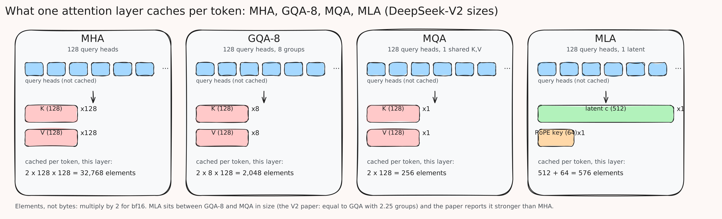
In multi-head attention with \(n_h\) heads of dimension \(d_h\), each token’s hidden state \(h_t \in \mathbb{R}^d\) is projected into per-head queries, keys, and values, and the keys and values of every past token are what decode reads. The DeepSeek-V2 paper states the cost directly: MHA “needs to cache \(2 n_h d_h l\) elements for each token” (section 2.1.1). With 128 heads of dimension 128 over 60 layers, that is 1.97 million elements per token, 3.9 MB in bf16.
The first fix predates DeepSeek. Multi-Query Attention (Shazeer, 2019) keeps \(n_h\) query heads but a single shared key head and value head, cutting the cache by a factor of \(n_h\) and, in the paper’s measurements, the per-step decoder time by roughly 12x. Grouped-Query Attention (Ainslie et al., 2023) interpolates: query heads are split into \(G\) groups, each sharing one K and one V head, so GQA-1 is MQA and GQA-\(n_h\) is MHA. Llama 3’s 8 KV heads are GQA-8. Both trade quality for cache; DeepSeek-V2’s own ablation on 7B models (Appendix D.1) has MMLU falling from 45.2 with MHA to 41.2 with GQA-8 and 37.9 with MQA.
MLA’s goal is the cache of MQA with the quality of MHA or better.
The latent
The idea is low-rank joint compression of K and V. Instead of projecting \(h_t\) into keys and values directly, project it into one small latent vector and derive both from that (V2 paper, equations 9 to 11):
\[c_t^{KV} = W^{DKV} h_t, \qquad k_t^{C} = W^{UK} c_t^{KV}, \qquad v_t^{C} = W^{UV} c_t^{KV}\]where \(c_t^{KV} \in \mathbb{R}^{d_c}\) is the latent, \(W^{DKV} \in \mathbb{R}^{d_c \times d}\) is the down-projection, and \(W^{UK}, W^{UV} \in \mathbb{R}^{d_h n_h \times d_c}\) are up-projections back to the full per-head keys and values. Only \(c_t^{KV}\) is cached: \(d_c\) elements per layer instead of \(2 n_h d_h\). For V2, \(d_c = 512\) against \(2 \times 128 \times 128 = 32{,}768\).
A second compression, of the queries through a latent \(c_t^Q\) of dimension \(d_c' = 1536\), is applied for the same reason on the query side, but it saves training activation memory rather than cache and can be ignored here.
Why RoPE breaks the trick, and the decoupled key
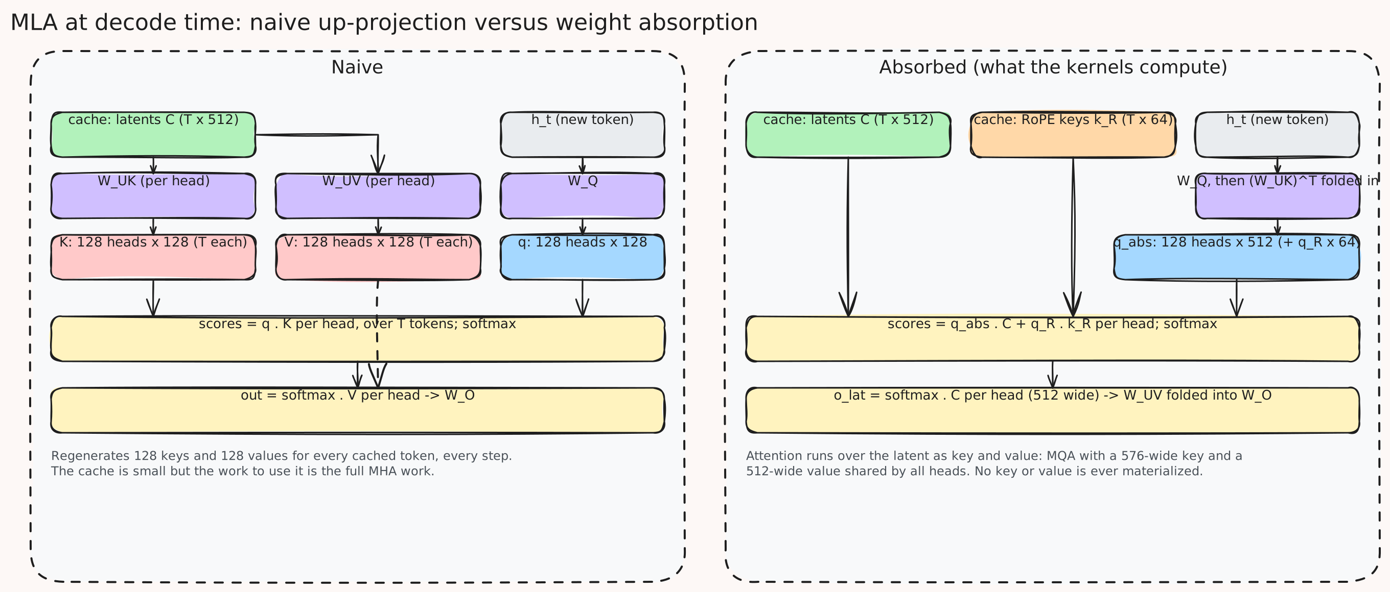
Caching a latent instead of keys only pays off if attention can be computed without regenerating the keys for every cached token at every step. It can, by associativity: the score between query \(q_{t,i}\) and key \(k_{j,i}\) of head \(i\) is
\[q_{t,i}^{\top} k_{j,i} = (W_i^{Q} h_t)^{\top} (W_i^{UK} c_j^{KV}) = \big[(W_i^{UK})^{\top} W_i^{Q} h_t\big]^{\top} c_j^{KV}\]so the up-projection \(W_i^{UK}\) can be folded into the query side once per step, and the cached latent is dotted directly. The paper calls this absorbing \(W^{UK}\) into \(W^Q\) (section 2.1.2 and Appendix C), and the same move on the value side folds \(W^{UV}\) into the output projection \(W^O\).
RoPE gets in the way. Rotary embeddings multiply queries and keys by a position-dependent rotation \(R_t\), and the rotation on the key sits between the two matrices being absorbed: with \(k_{j,i} = R_j W_i^{UK} c_j^{KV}\) the score becomes \(h_t^{\top} (W_i^{Q})^{\top} R_t^{\top} R_j W_i^{UK} c_j^{KV}\), and \(R_t^{\top} R_j = R_{j-t}\) depends on the position of every cached token. There is no single position-independent matrix to precompute. The paper’s words: “a RoPE matrix related to the currently generating token will lie between \(W^Q\) and \(W^{UK}\) and matrix multiplication does not obey a commutative law” (section 2.1.3).
The fix is to keep RoPE out of the compressed path entirely. A separate small decoupled key \(k_t^R \in \mathbb{R}^{d_h^R}\), shared across all heads, carries the positional information, alongside per-head decoupled queries \(q_{t,i}^R\) (equations 14 to 17):
\[k_t^{R} = \mathrm{RoPE}(W^{KR} h_t), \qquad q_{t,i} = [\,q_{t,i}^{C};\, q_{t,i}^{R}\,], \qquad k_{t,i} = [\,k_{t,i}^{C};\, k_t^{R}\,]\]The content part of the score absorbs as above; the RoPE part is a plain dot product against the cached \(k_j^R\). So the cache per token per layer is \(d_c + d_h^R\) elements, 512 plus 64 for V2, and the paper’s comparison table (Table 1) reads:
| Attention | Cached elements per token | Capability, per the paper |
|---|---|---|
| MHA | \(2 n_h d_h l\) | strong |
| GQA | \(2 n_g d_h l\) | moderate |
| MQA | \(2 d_h l\) | weak |
| MLA | \((d_c + d_h^R)\, l \approx 4.5\, d_h l\) | stronger |
With \(d_c = 4 d_h\) and \(d_h^R = d_h / 2\), MLA’s cache “is equal to GQA with only 2.25 groups, but its performance is stronger than MHA” (Table 1 caption).
Check it in numpy
The absorption claim is that the scores and outputs are identical whether you up-project the keys or fold the up-projection into the query. Twenty lines confirm it at toy sizes:
import numpy as np
rng = np.random.default_rng(0)
d, n_h, d_h, d_c, T = 64, 4, 16, 32, 10      # hidden, heads, head dim, latent dim, cached tokens
W_DKV = rng.standard_normal((d_c, d)) / np.sqrt(d)
W_UK  = rng.standard_normal((n_h, d_h, d_c)) / np.sqrt(d_c)
W_UV  = rng.standard_normal((n_h, d_h, d_c)) / np.sqrt(d_c)
W_Q   = rng.standard_normal((n_h, d_h, d)) / np.sqrt(d)
H = rng.standard_normal((T, d))              # hidden states of the cached tokens
h_t = rng.standard_normal(d)                 # the new query token
C = H @ W_DKV.T                              # (T, d_c): the only thing cached
# naive: up-project keys and values for every cached token, per head
K = np.einsum('hdc,tc->htd', W_UK, C)        # (n_h, T, d_h)
V = np.einsum('hdc,tc->htd', W_UV, C)
q = np.einsum('hdk,k->hd', W_Q, h_t)         # (n_h, d_h)
scores_naive = np.einsum('hd,htd->ht', q, K)
p = np.exp(scores_naive - scores_naive.max(1, keepdims=True)); p /= p.sum(1, keepdims=True)
out_naive = np.einsum('ht,htd->hd', p, V)    # (n_h, d_h)
# absorbed: fold W_UK into the query, attend over the latent, apply W_UV after
q_abs = np.einsum('hdc,hd->hc', W_UK, q)     # (n_h, d_c): one absorbed query per head
scores_abs = q_abs @ C.T                     # (n_h, T): keys are the raw latents
o_lat = p @ C                                # (n_h, d_c): values are the raw latents
out_abs = np.einsum('hdc,hc->hd', W_UV, o_lat)
print("max |score diff| :", np.abs(scores_naive - scores_abs).max())
print("max |output diff|:", np.abs(out_naive - out_abs).max())
print("cached floats per token, naive K+V:", 2 * n_h * d_h, " absorbed latent:", d_c)
Output on 2026-09-12 with numpy 2.4.1:
max |score diff| : 5.329070518200751e-15
max |output diff|: 6.661338147750939e-16
cached floats per token, naive K+V: 128  absorbed latent: 32
Differences at the level of floating-point rounding, and a cache four times smaller even at these toy sizes. The absorbed form is what every DeepSeek decode kernel since has computed, and it is why the FlashMLA support matrix describes DSA and CSA kernels as “MQA mode” with a 576- or 512-wide key: the latent is the key.
What V3 stored
DeepSeek-V3 kept MLA unchanged apart from the surrounding sizes: 61 layers, hidden 7168, 128 heads, and the same \(d_c = 512\), \(d_h^R = 64\) (V3 report, section 4.2; config.json). In bf16 the arithmetic is:
\[(512 + 64) \times 2 \text{ bytes} = 1{,}152 \text{ bytes per layer}, \qquad 1{,}152 \times 61 = 70{,}272 \text{ bytes per token}\]A 128K-token request therefore carries about 9.2 GB of cache. The FlashMLA deep dive quotes the same figure with the MTP layer included: \(576 \times 2 \times 62 \times 128 \times 1024 = 8.72\) GiB. For comparison, MHA with V3’s head geometry would be \(128 \times 192 \times 2 \times 2 = 98{,}304\) bytes per layer, 6.0 MB per token, 85 times more. GQA-8 with the same heads would be 375 KB per token, still 5.3 times more.
References
- DeepSeek-V2: A Strong, Economical, and Efficient Mixture-of-Experts Language Model, sections 2.1 and Appendix C, Table 1, Appendix D
- DeepSeek-V3 Technical Report, section 4.2; DeepSeek-V3 config.json
- Fast Transformer Decoding: One Write-Head is All You Need, Shazeer 2019; GQA, Ainslie et al. 2023
- FlashMLA Hopper FP8 sparse deep dive
Sliding Window Attention
MLA shrinks the entry. The next lever shrinks the count of entries, and the simplest way to do that is to forget: let each token attend only to the \(W\) tokens before it. This section is short because the idea is old, but V4 puts a window in every layer and V4.1’s replay trick depends on how far a stack of windows can see, so the details matter later.
Definition and the bounded cache
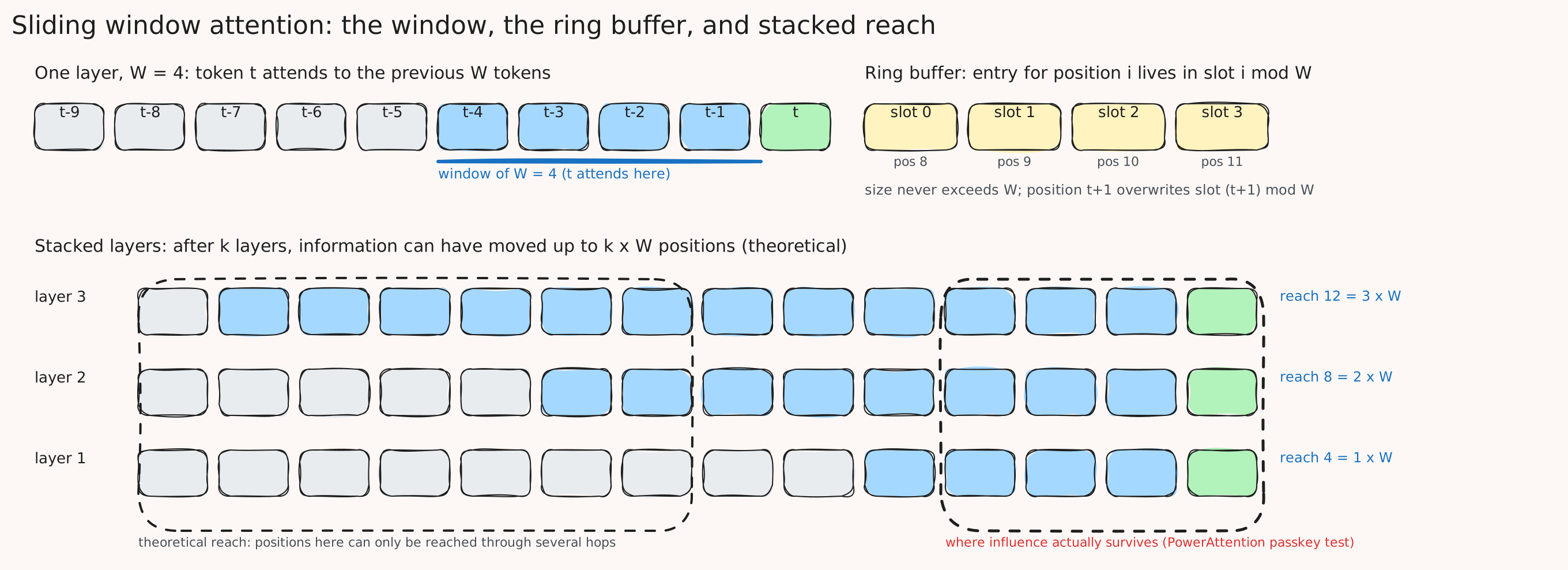
Longformer (Beltagy et al., 2020) defined the pattern: “Given a fixed window size \(w\), each token attends to \(\tfrac{1}{2}w\) tokens on each side,” with cost \(O(n \times w)\), linear in sequence length. In a causal decoder the window is entirely to the left. Mistral 7B (Jiang et al., 2023) made the cache consequence explicit: “the cache has a fixed size of \(W\), and the keys and values for the timestep \(i\) are stored in position \(i \bmod W\) of the cache,” a rolling buffer that stops growing once \(i > W\). At Mistral’s \(W = 4096\) that cuts the cache 8x on a 32K sequence.
So a sliding-window layer’s cache is \(W\) entries, full stop, whatever the context. That is why DeepSeek’s per-token figures exclude it, and why the V4.1 report can say the sliding-window cache “is bounded independently of sequence length” while everything else scales.
Stacked windows see further, but not as far as the arithmetic says
Windowed layers stack. Longformer: “In a transformer with \(\ell\) layers, the receptive field size at the top layer is \(\ell \times w\).” Mistral restates it as a decoder: “after \(k\) attention layers, information can move forward by up to \(k \times W\) tokens,” which at 32 layers and \(W = 4096\) is a theoretical span of 131K tokens.
That theoretical span is the number you should distrust, and the V4.1 report does. When it argues that replaying only the last window of tokens is enough to rebuild the sliding-window cache, its justification is that “the actual effective receptive field of SWA is much smaller than the theoretical \(n_{win} \times L/2\),” citing PowerAttention (Chen et al., 2025). PowerAttention’s evidence is a passkey-retrieval experiment rather than a formula: with a window of about 2K tokens, sliding-window models “perform well up to 12K tokens but degrade significantly at 16K and 32K,” and the authors estimate the information strength “decays to near zero after propagating through 6 layers.” The exact reach depends on the model, but the shape of the finding is what the later trick relies on: the influence of a token through stacked windows fades after a few hops, so the entries far back in the theoretical span carry little, and an approximate reconstruction from the last window loses little.
References
- Longformer: The Long-Document Transformer, Beltagy et al. 2020, section 3.1
- Mistral 7B, Jiang et al. 2023, section 2
- PowerAttention: Exponentially Scaling of Receptive Fields for Effective Sparse Attention, Chen et al. 2025
- DeepSeek-V4.1-Flash tech report, sections 2.2 and 3.2.2
DeepSeek-V3.2: Sparse Attention With a Learned Indexer
The cost: every query reads every latent
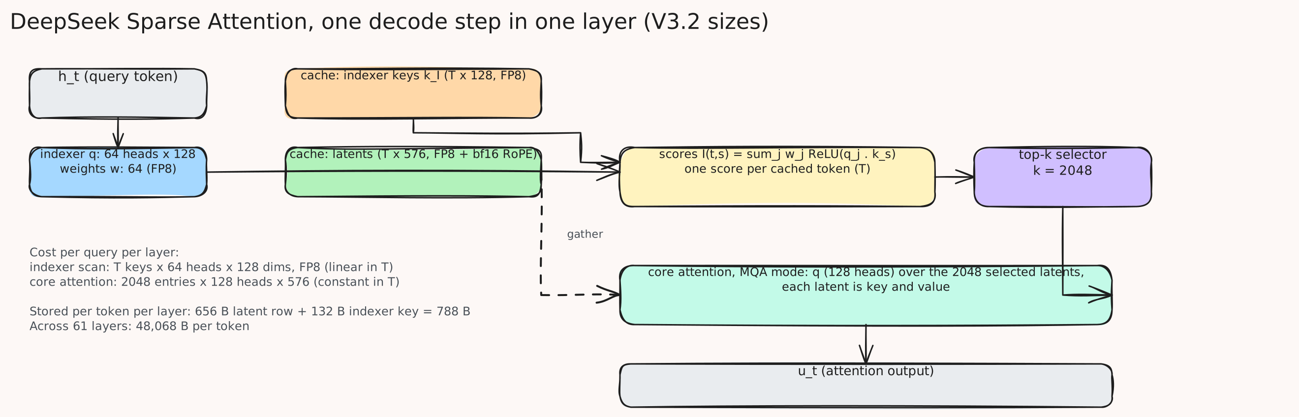
MLA made the entry small, but at 128K context a decode step still reads 128K latents per layer per query and multiplies against all of them. The cache is \(O(L)\) in context length and so is the work; at long context the work is what hurts, and it is \(O(L^2)\) over a full prefill. A window bounds the work but throws away the far context. DeepSeek Sparse Attention (DSA), introduced in DeepSeek-V3.2-Exp in September 2025 and kept unchanged in V3.2, keeps the far context available and reads only the useful part of it: a cheap scorer ranks every cached entry for the current query, and attention touches only the top \(k\).
The lightning indexer
The scorer is a tiny attention of its own. For query token \(t\) and cached token \(s\), the V3.2-Exp tech report defines the index score (equation 1):
\[I_{t,s} = \sum_{j=1}^{H^I} w^{I}_{t,j} \cdot \mathrm{ReLU}\big(q^{I}_{t,j} \cdot k^{I}_{s}\big)\]with \(H^I\) indexer heads, per-head indexer queries \(q^I_{t,j} \in \mathbb{R}^{d^I}\) and scalar weights \(w^I_{t,j}\) derived from \(h_t\), and a single shared indexer key \(k^I_s \in \mathbb{R}^{d^I}\) per cached token. Three design choices are visible in the formula. The key has no head index, so the indexer is itself MQA-shaped and caches one small vector per token. ReLU rather than softmax, “for throughput consideration.” And it runs in FP8: “given that the lightning indexer has a small number of heads and can be implemented in FP8, its computational efficiency is remarkable.” In V3.2 the indexer has 64 heads of dimension 128, from config.json, against the main attention’s 128 heads of 192.
Selection is then a top-\(k\) over the scores, with \(k = 2048\) (equation 2, index_topk):
The \(c_s\) are the MLA latents. DSA is “instantiated based on the MQA mode of MLA, where each latent vector will be shared across all query heads,” because “each key-value entry must be shared across multiple queries for computational efficiency” at the kernel level. The absorbed form from the previous section is not an optimization any more; it is the representation the sparse kernel selects over.
What it costs and what it saves
Complexity, from the report’s section 3: “DSA reduces the core attention complexity of the main model from \(O(L^2)\) to \(O(Lk)\) … Although the lightning indexer still has a complexity of \(O(L^2)\), it requires much less computation compared with MLA.” The indexer is the piece that still scales, and the entire V4 and V4.1 story of compressed keys, FP4 indexer math, and candidate pools is about making that one scan cheaper. Per token, V3.2 stores the 576-wide latent in FP8 and the 128-wide indexer key in FP8, which the FlashMLA README lays out as a 656-byte row (512 bytes of FP8 latent, 16 bytes of four FP32 scales, 128 bytes of bf16 RoPE key) plus, per the V4.1 chart’s arithmetic, 132 bytes for the indexer key and its scale. Across 61 layers: \(61 \times (656 + 132) = 48{,}068\) bytes per token, the second bar on the chart.

How the indexer learns what attention wants
The indexer is trained to imitate the dense attention it replaces, in two stages (report, section 2.1). First, with dense attention still on and every other parameter frozen, the model’s real attention scores are summed over heads and L1-normalized per query into a target distribution \(p_{t,:}\), and the indexer minimizes \(\sum_t D_{KL}(p_{t,:} \,\|\, \mathrm{Softmax}(I_{t,:}))\) for 1,000 steps on 2.1B tokens. Then sparse attention is switched on, the KL target is restricted to the selected set, and everything trains together for 943.7B tokens, with the indexer’s input detached from the main graph so that its only signal is the imitation loss. The result on benchmarks is within noise of the dense model (Table 1 of the report), which is what makes the rest of the lineage possible: from here on, attention reads a learned subset, and the subset can be made cheaper to find.
References
- DeepSeek-V3.2-Exp: Boosting Long-Context Efficiency with DeepSeek Sparse Attention; DeepSeek-V3.2 report, section 2
- DeepSeek-V3.2-Exp model card and config.json
- FlashMLA README; DeepGEMM (indexer logit kernels); DeepSelect (top-k kernel)
A Precision Primer
The next two generations quantize the cache, first to FP8 with bf16 exceptions, then to FP4. The formats have names that look like part numbers, so here is what each one is, with the numbers that matter for a cache.
FP8: E4M3 and E5M2
An 8-bit float spends its bits on a sign, an exponent field, and a mantissa field. The FP8 paper (Micikevicius et al., 2022) defines the two layouts everyone uses:
| E4M3 | E5M2 | |
|---|---|---|
| Bits | 1 sign, 4 exponent, 3 mantissa | 1 sign, 5 exponent, 2 mantissa |
| Max finite | 448 | 57,344 |
| Min subnormal | \(2^{-9}\) | \(2^{-16}\) |
| Infinities | not represented | yes |
| NaN | one bit pattern | IEEE style |
E4M3 trades range for precision and bends IEEE conventions to get one more binade: infinities are dropped and only a single NaN encoding is kept, which “extends the dynamic range by one extra power of 2, from 17 to 18 binades.” For a cache of normalized activations, where values live within a few orders of magnitude, E4M3 is the right one, and it is what every DeepSeek FP8 cache uses.
Block scaling: MX formats and E8M0
Four bits cannot cover a useful range alone, so low-bit formats share a scale across a block of elements. The OCP Microscaling paper (Rouhani et al., 2023) fixes the convention: “A basic unit of data in an MX format represents a vector of \(k\) numbers and consists of a single shared scale \(X\) and \(k\) scalar elements,” decoded as \(v_i = X P_i\), with \(k = 32\) and the scale stored as E8M0, an 8-bit exponent with no mantissa, so every scale is a power of two from \(2^{-127}\) to \(2^{127}\) (CUDA docs). The concrete formats:
| Format | Element | Block | Scale | Bits per element with scale |
|---|---|---|---|---|
| MXFP8 | E4M3 or E5M2 | 32 | E8M0 | 8.25 |
| MXFP6 | E2M3 or E3M2 | 32 | E8M0 | 6.25 |
| MXFP4 | E2M1 | 32 | E8M0 | 4.25 |
| NVFP4 | E2M1 | 16 | E4M3, plus one FP32 per tensor | 4.5 |
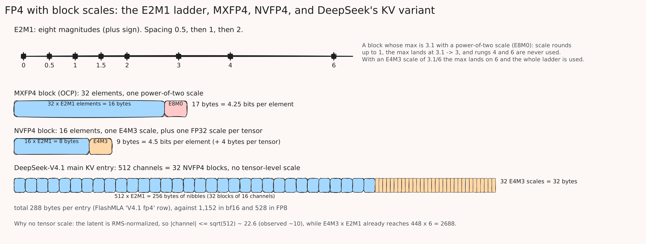
The bits-per-element column is element bits plus scale bits divided by block size, so MXFP4 is \(4 + 8/32 = 4.25\) and NVFP4 is \(4 + 8/16 = 4.5\). The UE8M0 you see in DeepSeek configs is this E8M0 scale, unsigned; DeepSeek-V3.1’s card says the model “is trained using the UE8M0 FP8 scale data format on both model weights and activations to ensure compatibility with microscaling data formats” (V3.1 model card).
E2M1: eight magnitudes
The FP4 element is E2M1: a sign, two exponent bits, one mantissa bit. That gives exactly eight magnitudes, “\(\pm 0, \pm 0.5, \pm 1, \pm 1.5, \pm 2, \pm 3, \pm 4, \pm 6\)” (NVFP4 paper, section 2), with no infinity and no NaN (CUDA docs). Notice the spacing: 0.5 apart up to 2, then 1 apart, then 2 apart. Everything about FP4 accuracy is about placing the block’s values onto that ladder well, and that is the scale’s job.
NVFP4: why a fractional scale beats a power of two
NVIDIA’s NVFP4 changes three things relative to MXFP4 (NVFP4 paper, section 2): blocks of 16 instead of 32, so each scale covers a narrower range of values; an E4M3 scale instead of E8M0, so the scale can be any value with three mantissa bits rather than only a power of two; and a second, per-tensor FP32 scale to restore the range the E4M3 scale gave up. The paper’s worked example says why the mantissa bits matter. If a block’s largest magnitude is \(3 + \delta\), the ideal scale is \((3 + \delta)/6\), just over 0.5. E8M0 must round that up to 1, so after scaling the block’s maximum lands at \(3 + \delta\), which quantizes to 3, and the top two rungs of the ladder, 4 and 6, go unused: “only \(\log_2(3/0.5) = 2.58\) binades are utilized instead of the full \(\log_2(6/0.5) = 3.58\) binades.” An E4M3 scale lands the maximum near 6 and uses the whole ladder.
Two-level range: an E4M3 scale times an E2M1 value reaches at most \(448 \times 6 = 2688\), and the FP32 tensor scale maps whatever the tensor’s actual maximum is onto that ceiling. Hold onto the 2688; the V4.1 section uses it to explain why DeepSeek’s FP4 cache drops the tensor-level scale.
What the hardware multiplies
On Blackwell, all of these are native matmul operands: the PTX ISA’s block-scaled mma kinds cover E4M3, E5M2, E2M3, E3M2, and E2M1 elements with E8M0 scales at block 32, and E2M1 with E4M3 scales at block 16 (PTX ISA, block scaling). The NVFP4 paper’s table gives the throughput multipliers over bf16: 2x for MXFP8 and MXFP6, 4x for MXFP4 and NVFP4 on GB200, 6x on GB300. A cache in FP4 does not need any of that, though. The V4.1 report is careful on this point: for the main KV cache “FP4 reduces storage rather than accelerates matrix multiplication,” because the cached values are dequantized before attention, which “preserv[es] compatibility across hardware platforms.” Only the indexer’s query-key product actually multiplies in FP4.
References
- FP8 Formats for Deep Learning, Micikevicius et al. 2022, Table 1
- Microscaling Data Formats for Deep Learning, Rouhani et al. 2023, section 2 and Table 1
- Pretraining Large Language Models with NVFP4, NVIDIA 2025, section 2 and Appendix B; Introducing NVFP4, NVIDIA developer blog
- CUDA Math API: E8M0, E2M1; PTX ISA
- DeepSeek-V3.1 model card; DeepSeek-V4.1-Flash tech report, section 2.4.4
DeepSeek-V4: Compress the Sequence, Then Sparsify
DeepSeek-V4 (April 2026) is where the context target becomes one million tokens, and the report’s own framing is that “as the context length reaches extreme scales, the attention mechanism emerges as the dominant computational bottleneck.” V3.2’s DSA left two costs growing linearly with context: the indexer’s scan over every cached token, and the cache itself at 48 KB per token. V4 attacks both by changing what a cache entry represents. An entry is no longer one token; it is a compressed summary of several. Three attention variants share the model, each with its own compression ratio, and every layer additionally keeps a sliding window. The result, from the report’s Figure 1: at 1M context, V4-Flash needs 10% of V3.2’s single-token FLOPs and 7% of its KV cache.

A window in every layer
Every CSA and HCA layer in V4 has a supplementary sliding-window branch of \(n_{win} = 128\) uncompressed entries, and the report gives two reasons (section 2.3.3). Compressed entries only exist for completed blocks, so “a query cannot access information from other tokens within its own compressed block” without it. And “recent tokens usually possess greater relevance.” In the core attention the 128 window entries are simply concatenated with the selected compressed entries, so a query in V4-Flash attends to 512 compressed entries plus 128 recent tokens. Layers with compression ratio 0 in the config are pure sliding-window layers: the first two in V4-Flash.
Compressed Sparse Attention: 2m tokens into one entry
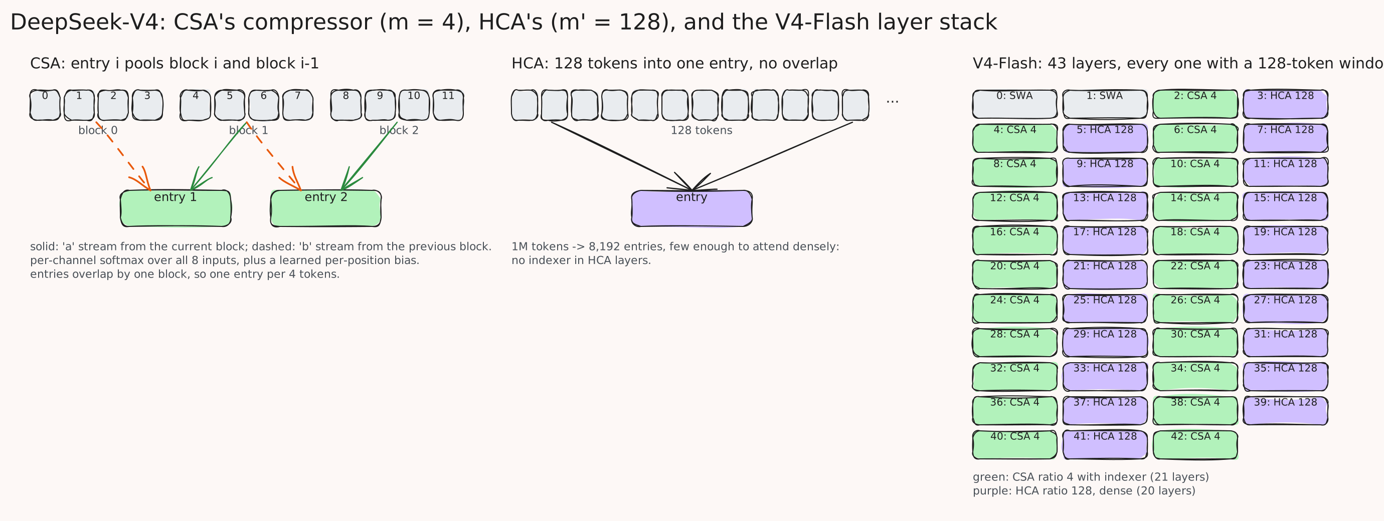
CSA “first compresses the Key-Value cache of every \(m\) tokens into one entry, and then applies DeepSeek Sparse Attention where each query token attends to only \(k\) compressed KV entries.” The compressor (section 2.3.1, equations 9 to 12) is a learned, gated pooling. From the hidden states \(H\) it computes two candidate-entry streams and two gate streams with four \(d \times c\) projections:
\[C^a = H W^{aKV}, \quad C^b = H W^{bKV}, \quad Z^a = H W^{aZ}, \quad Z^b = H W^{bZ}\]and forms compressed entry \(i\) from the current block of \(m\) tokens through the \(a\) stream and the previous block through the \(b\) stream:
\[C^{Comp}_i = \sum_{j=mi}^{m(i+1)-1} S^a_j \odot C^a_j \;+\; \sum_{j=m(i-1)}^{mi-1} S^b_j \odot C^b_j\]where the gates \(S\) are a softmax over all \(2m\) inputs of \(Z + B\), with \(B^a, B^b \in \mathbb{R}^{m \times c}\) learnable biases that encode a token’s position within its block. Two details matter. The softmax and the product are per channel (the \(\odot\) is a Hadamard product), so each of the \(c = 512\) output channels chooses its own mix of the \(2m\) inputs. And the two-block window overlaps: entry \(i\) reads blocks \(i\) and \(i-1\), entry \(i-1\) reads blocks \(i-1\) and \(i-2\), so “CSA in fact compresses the sequence length to \(1/m\) times” even though each entry sees \(2m\) tokens. V4 uses \(m = 4\).
The indexer then scores compressed entries rather than tokens. Indexer keys are produced by “the same compression operation used for \(C^{Comp}\),” the score is the V3.2 formula over compressed positions (equation 16), and top-\(k\) selects \(k = 512\) entries for V4-Flash, which at ratio 4 cover the same 2048 raw positions that V3.2’s top-2048 did. Core attention is MQA where “each compressed KV entry serves as both attention key and value” (equation 19): there is one 512-wide vector per entry, no separate value, num_key_value_heads: 1.
Heavily Compressed Attention: ratio 128, no indexer
HCA is the same compressor without the overlap and with \(m' = 128\), and it “does not employ sparse attention” (section 2.3.2). At ratio 128 a million-token context is 8,192 entries, few enough to attend densely, so there is nothing for an indexer to select. In V4-Flash the layers alternate: config compress_ratios is [0, 0, 4, 128, 4, 128, ..., 4], two window-only layers then 21 CSA and 20 HCA layers.
Three details that make the single vector work
Using one vector as both key and value, and rotating it, needs three fixes (section 2.3.3):
| Detail | What | Why |
|---|---|---|
| Normalization | an RMSNorm on each query head and on the single compressed entry, just before attention | bounds the magnitudes, which is what makes the FP4 range argument in the next section work |
| Partial RoPE with un-rotation | RoPE on the last 64 dimensions of the query and the entry; then RoPE with position \(-i\) on the last 64 dimensions of each head’s output | the entry is also the value, so the rotated dimensions would leak absolute position into the output; rotating back cancels it |
| Attention sinks | a learnable per-head logit \(z'_h\) whose exponential is added to the softmax denominator | lets a head put attention mass “nowhere,” so its total can be below 1 or near 0 |
The un-rotation is the reason FlashMLA’s V4 kernels are described as fusing “Q-RoPE, core attention, O-RoPE (conjugate).”
The indexer in four bits
V4’s indexer keys and queries are quantized to MXFP4 with quantization-aware training: “the Query-Key path in the indexer of CSA, where QK activations are cached, loaded, and multiplied entirely in FP4” (section 5.2.1). This is the one place FP4 arithmetic, not just FP4 storage, is used, and it is the piece of V3.2’s \(O(L^2)\) scan that could be made cheaper per element. The report adds that index scores were cut from FP32 to bf16 for “a 2x speedup for the top-k selector, while preserving a 99.7% recall rate.”
What V4 stores per token
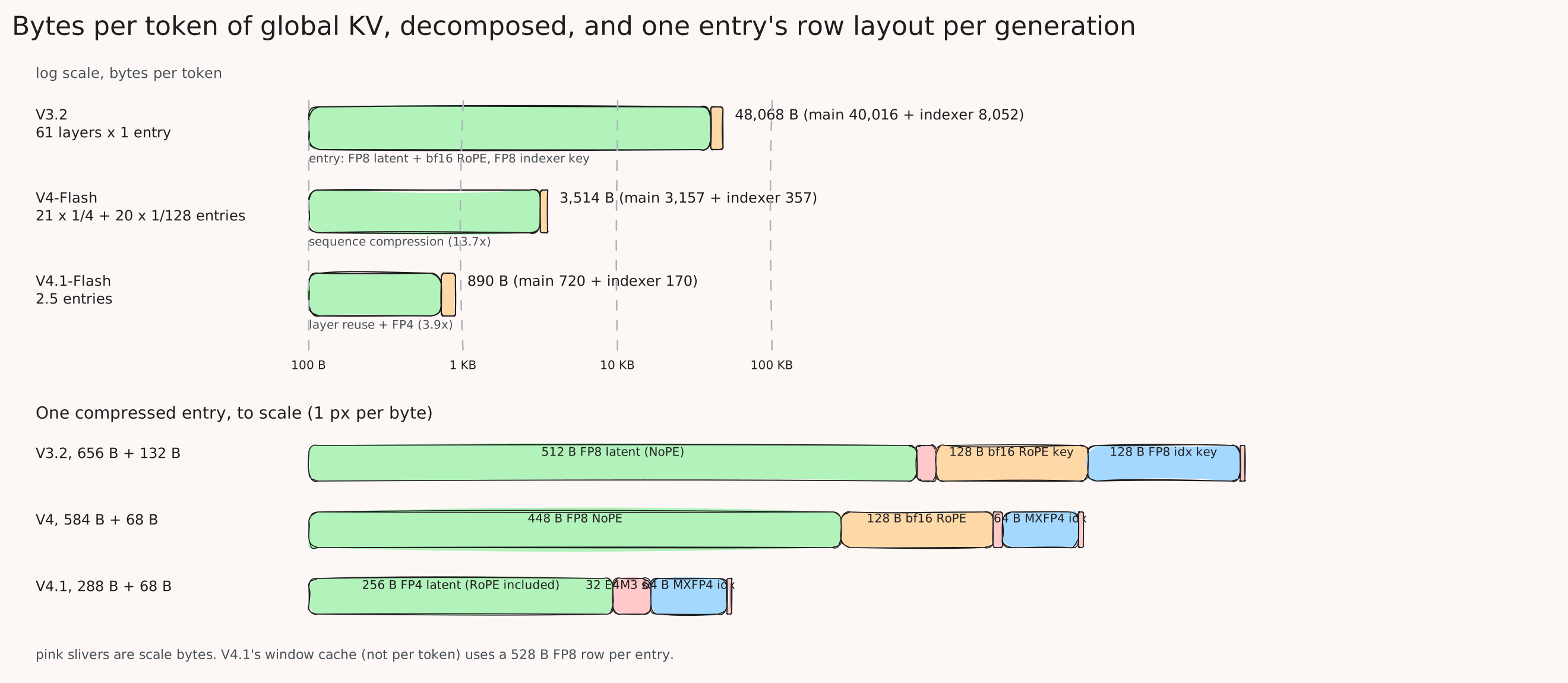
Per compressed entry, FlashMLA’s V4 row is 584 bytes: 448 bytes of FP8 for the non-RoPE part, 128 bytes of bf16 for the 64 RoPE dimensions, which are kept in bf16 “for accuracy,” and 8 bytes of E8M0 scales. The report’s description matches: “BF16 precision is used for the RoPE dimensions, while FP8 precision is applied to the remaining dimensions,” which “reduces the KV cache size by nearly half compared with pure BF16.” The MXFP4 indexer key is \(128 \times 0.5 = 64\) bytes plus four E8M0 scales, 68 bytes. So for V4-Flash:
\[21 \times \frac{584 + 68}{4} \;+\; 20 \times \frac{584}{128} = 3{,}423 + 91 \approx 3{,}514 \text{ bytes per token}\]which is the third bar on the chart, and the 13.7x against V3.2’s 48,068 that the report’s Figure 1 labels. The sliding-window branch adds 128 entries of 584 bytes per layer, about 3 MB per sequence, bounded.
The cache that does not fit the page table, and Zero SWA Caching
Two serving consequences appear in the report’s inference section (3.5) and both return in V4.1. First, the cache has two shapes. Compressed entries are a classical paged cache. The window entries and the not-yet-compressed tail tokens are a fixed-size per-request block that the report treats “as a state-space model”: pre-allocated, bounded, and not paged. Second, persistence. DeepSeek stores prefixes on SSD for reuse across requests, and compressed entries store well because everything past the last complete block is reusable. Window entries do not: they “exist in every layer” uncompressed, so their volume “is approximately 8 times larger than the compressed CSA and HCA KV entries,” and only the last 128 per layer are ever needed. The report weighs three options and names the one it will pursue: Zero SWA Caching, store no window entries at all, and on a prefix hit rebuild them by recomputing. The catch is the cost of an exact rebuild: because each layer’s window depends on the previous layer’s window, “recomputing the last \(n_{win} \cdot L\) tokens is enough to restore the last \(n_{win}\) SWA KV entries for an \(L\)-layer model.” For V4-Flash that is \(128 \times 43 = 5{,}504\) tokens of recomputation on every cache hit. V4.1’s bounded replay is the answer to exactly this number.
References
- DeepSeek-V4: Towards Highly Efficient Million-Token Context Intelligence, sections 2.3, 3.5, 4.2.1, 5.2.1, Figure 1
- DeepSeek-V4-Flash model card and config.json
- FlashMLA README, FP8 KV cache section and support matrix
DeepSeek-V4.1: Reuse Across Layers, Project Across Halves, Store in Four Bits
DeepSeek-V4.1-Flash (September 2026) is titled “Pushing the Limits of KV Cache Compression,” and after V4 the remaining levers were the layer dimension and precision. It pulls both, and adds a structural change to what prefill has to compute. The model is 40 layers at hidden size 5120, with 552B backbone parameters, and every attention layer is the V4 design with three modifications: a simplified compressor called CSA2, a static assignment of every layer to one of three reuse modes, and a split of the network into a causal encoder and a decoder.
CSA2: the simplified compressor
Three simplifications relative to V4’s CSA (report, section 2.3): the compressor no longer overlaps source windows, so an entry pools exactly its own \(m\) tokens; the learned position bias inside the block is dropped; and the indexer key is projected from the main KV entry rather than compressed separately from the hidden states. The last one is what makes cross-layer reuse cheap, because a layer that borrows another’s main KV gets its indexer keys along with it. Compression ratios also change: the encoder layers use \(m = 2\), the decoder layers use \(m = 1\), uncompressed, and HCA is gone entirely, “pure CSA2.” Top-\(k\) stays 512 and the indexer shrinks to 32 heads of 128.
Three modes
Every CSA2 layer is statically one of Full, Reindex, or Reuse (section 2.3.1). All three compute their own query and their own 128-token window; they differ in where the expensive pieces come from:
| Mode | Main KV | Indexer K | Top-K indices | Computes |
|---|---|---|---|---|
| Full | its own | projected from its own KV | runs the indexer | everything |
| Reindex | reused from the most recent Full layer | reused | its own indexer Q, rescored, fresh top-K | query, window, indexer Q and scoring |
| Reuse | reused | reused | reused from the latest Full or Reindex layer | query and window only |
The two reuses are decoupled on purpose. Sharing main KV divides the cache by the group size. Reusing top-K divides the indexer work. Reindex mode keeps the first saving while letting the selection change, so the model can look at different entries in different layers without storing different entries. The report cites the prior work that tried each half separately, IndexCache for index reuse, YOIO for a single shared routing, HySparse for KV sharing from dense layers, and argues none covered all three dimensions at once.
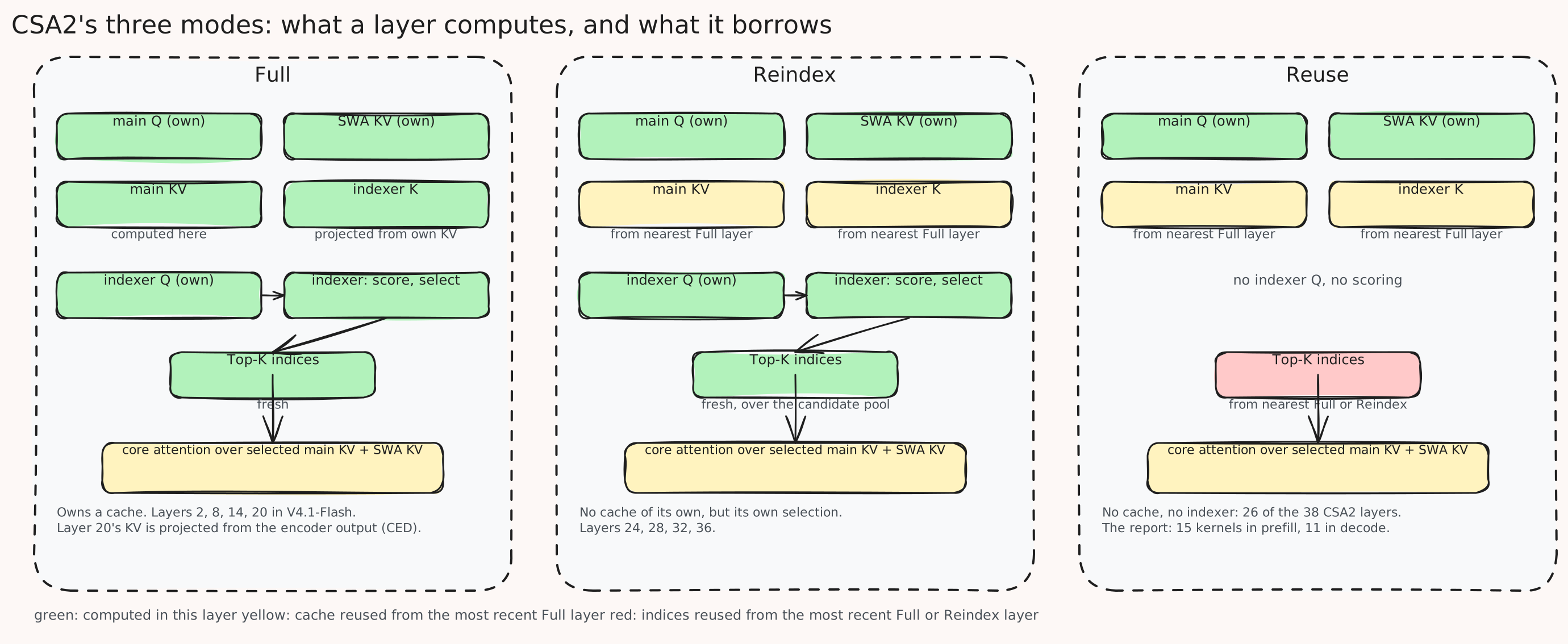
The assignment for V4.1-Flash, from section 4.2.1 and confirmed by kv_source_layer_ids and index_source_layer_ids in config.json:
| Layers | Ratio | Modes |
|---|---|---|
| 0, 1 | window only | |
| 2 to 7, 8 to 13, 14 to 19 | 2 | first of each six Full, the other five Reuse |
| 20 to 23 | 1 | Full, then three Reuse |
| 24 to 27, 28 to 31, 32 to 35, 36 to 39 | 1 | Reindex, then three Reuse |
Four layers write a main KV cache. Eight run an indexer. Twenty-six do neither. The per-token consequence, which the arithmetic section finishes: a token adds one entry at layer 20 and half an entry at each of layers 2, 8, and 14, so 2.5 entries across the whole network, against V4-Flash’s 21 quarter-entries and 20 one-hundred-twenty-eighth entries.
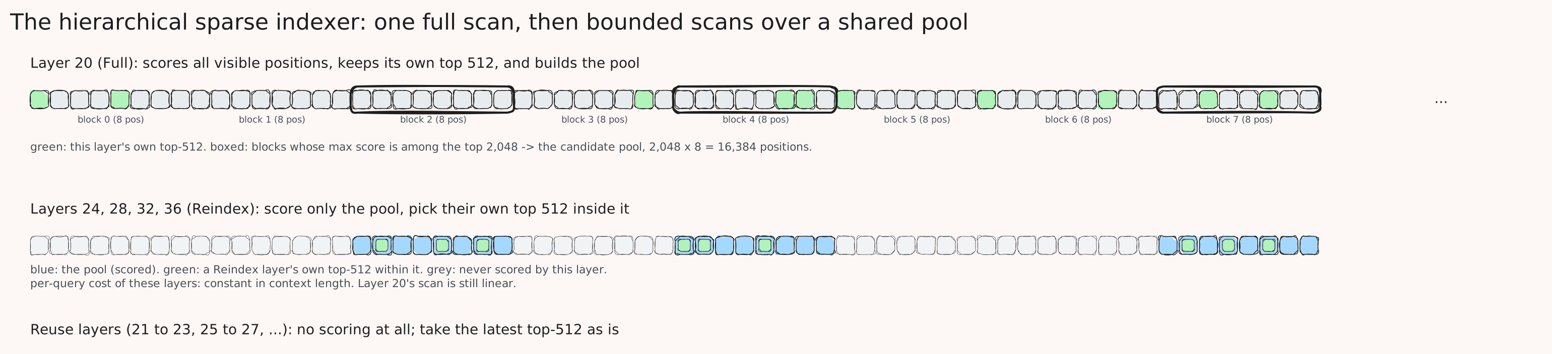
The hierarchical indexer
Index reuse cut the number of layers that scan; it did not shorten the scan. The decoder’s first Full layer, layer 20, still scores every visible position, and the four Reindex layers above it would too. The hierarchical sparse indexer (section 2.3.2) bounds them. Layer 20 does its full scan and picks its own top 512. It also scores each block of 8 positions by the maximum score inside it, keeps the top 2,048 blocks, and publishes those \(2{,}048 \times 8 = 16{,}384\) positions as a candidate pool. Layers 24, 28, 32, and 36 score only the pool. “For a fixed candidate-pool size, this changes the per-query cost of deeper indexers from linear in context length to constant.” The first full scan remains, so the indexer cost at 1M context is one full scan plus four bounded ones, and the restriction was introduced in post-training so that “deeper indexers are optimized under the same search domain they use at inference.”
The causal encoder-decoder
The cache levers so far were about decode. Prefill, which in agentic use re-sends a growing context on every tool call, was still a full 40-layer pass. The causal encoder-decoder (CED, section 2.2) halves it, and the idea comes from YOCO (Sun et al., 2024), whose “decoder-decoder” design has a self-decoder produce one global KV cache that the cross-decoder layers above it reuse, so that “we can exit early before entering the cross-decoder during the prefill stage.” YOCO reported “at least half prefilling latency reduction.”
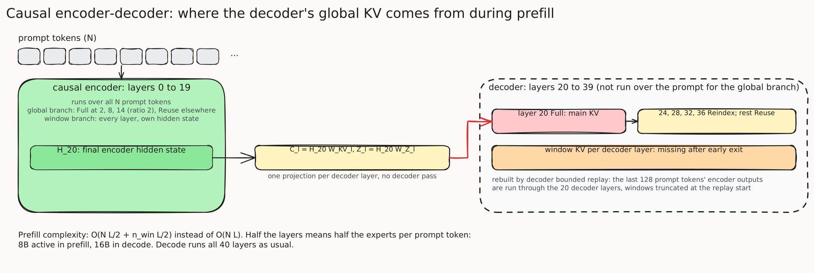
CED applies this to the global branch and keeps the window branch layer-local. The bottom 20 layers are the causal encoder. For the decoder layers \(l > L/2\), the main KV entries are not derived from that layer’s hidden state; they are projected from the encoder’s final hidden state with layer-specific weights (equation 1):
\[C^l = H_{L/2} W^{KV}_l, \qquad Z^l = H_{L/2} W^{Z}_l, \qquad l > L/2\]So once the encoder has run over the prompt, every decoder layer’s global cache can be filled with one projection each, no decoder forward pass needed. The report’s prefill complexity is \(O(NL/2 + n_{win} L/2)\) for a prompt of \(N\) tokens. That is where the model card’s “8B parameters per token during prefill and 16B during decode” comes from: prefill runs half the layers and therefore half the experts. The window branch is the exception, computed in every layer from that layer’s own hidden state, and it is the remaining \(n_{win} L/2\) term, which the next subsection deals with.
Four bits for the main KV, eight for the window
V4 stored the main entry as FP8 with bf16 RoPE dimensions. V4.1 stores it as FP4 (section 2.4.4): E2M1 elements with one E4M3 scale per 16 channels, “following NVFP4 but omitting its second-level global scale.” The argument for dropping the tensor-level scale is a bound. The largest trained RMSNorm weight is about 1, so after the normalization from V4’s “three details” the 512-channel latent has L2 norm at most about \(\sqrt{512} \approx 22.6\); RoPE is a rotation and preserves it; so no channel can exceed 22.6 in magnitude, and the observed maximum in training is around 10. The block format without a global scale already reaches \(448 \times 6 = 2688\), “far above the cache’s magnitude bound,” so the global scale would only add complexity. Quantization happens after RoPE, because quantizing before it “would introduce additional overhead during decoding.” The main cache goes to four bits with QAT in post-training; the window cache stays FP8 “due to its sensitivity to quantization”; the indexer keys stay MXFP4 for hardware portability.
Per compressed entry: \(512 \times 0.5 = 256\) bytes of nibbles plus 32 scale bytes, 288 bytes, matching FlashMLA’s “V4.1 fp4” row. The FP8 window entry is 528 bytes: 512 bytes of E4M3, RoPE dimensions included, plus 16 E8M0 scales.
Check it in numpy
The range argument says a normalized latent fits the E2M1 ladder comfortably; the ladder’s coarseness says the error will not be tiny. A fifteen-line quantizer applied to a random 512-channel vector normalized to L2 norm \(\sqrt{512}\), in blocks of 16 with an E4M3 scale that maps each block’s maximum onto 6:
import numpy as np
E2M1 = np.array([0, .5, 1, 1.5, 2, 3, 4, 6])          # the eight FP4 magnitudes
def to_e4m3(s):                                          # round a positive scale to an E4M3 value
    e = np.floor(np.log2(s)); m = np.round(s / 2**e * 8) / 8   # 3 mantissa bits
    return min(m * 2**e, 448.0)
def quant_block(x):                                      # x: 16 channels sharing one scale
    scale = to_e4m3(np.abs(x).max() / 6.0)               # map the block max onto 6.0
    y = x / scale
    idx = np.abs(np.abs(y)[:, None] - E2M1).argmin(1)    # nearest magnitude
    return np.sign(y) * E2M1[idx] * scale
rng = np.random.default_rng(0)
latent = rng.standard_normal(512); latent *= np.sqrt(512) / np.linalg.norm(latent)   # RMSNorm-like: L2 norm sqrt(512)
deq = np.concatenate([quant_block(b) for b in latent.reshape(32, 16)])
err = deq - latent
print("max |latent|       :", np.abs(latent).max().round(3))
print("rel L2 error       :", (np.linalg.norm(err) / np.linalg.norm(latent)).round(4))
print("bytes per 512-ch entry: fp16", 512*2, " fp8", 512, " fp4+E4M3/16", 512//2 + 32)
Output on 2026-09-12:
max |latent|       : 3.861
rel L2 error       : 0.0912
bytes per 512-ch entry: fp16 1024  fp8 512  fp4+E4M3/16 288
A Gaussian latent’s maximum sits near 4, nowhere near the 22.6 bound. The relative error of about 9% is the price of eight magnitudes per block, and it is why the format needs quantization-aware training rather than a post-hoc cast, and why the window cache, which the report found sensitive, stays at eight bits. This toy ignores the E4M3 rounding of the scale in the way the real kernel does it and uses round-to-nearest on the ladder, so treat the 9% as the order of magnitude, not the model’s number.
Bounded replay
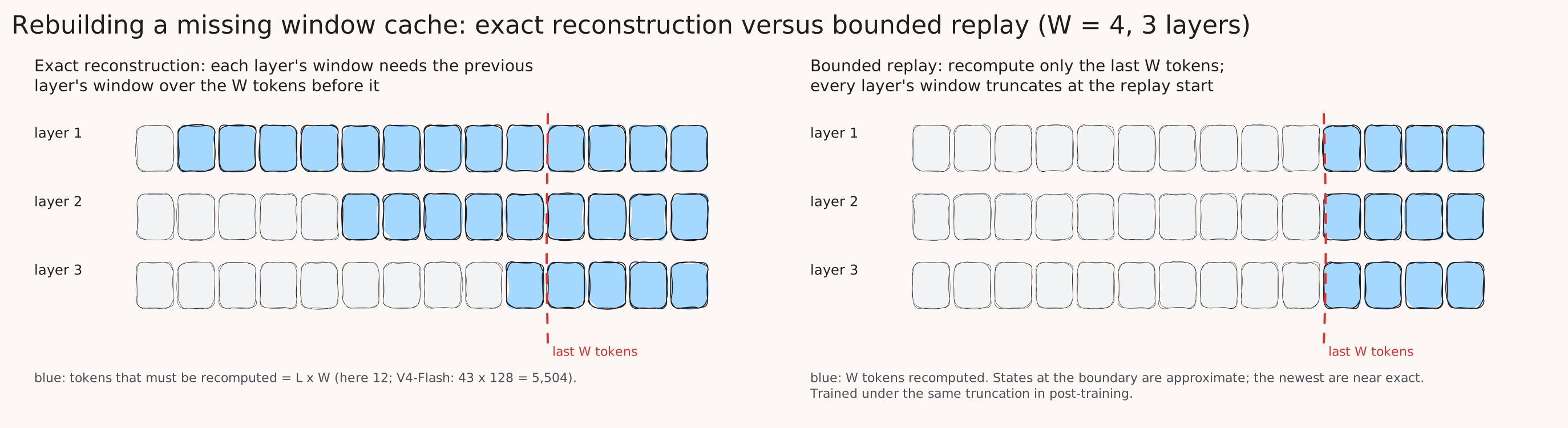
Two places in the design need window entries that nobody stored. On a persistent-cache hit, the encoder’s window entries were deliberately not persisted (V4’s Zero SWA Caching). After CED’s early exit, the decoder’s window entries were never computed. Exact reconstruction costs \(L \times n_{win}\) tokens of recomputation in both cases, because window states chain through the layers.
SWA Bounded Replay (section 3.2.2) replays only the last \(n_{win} = 128\) tokens and truncates every layer’s window to that segment: for a replay starting at position \(s\), a query at \(i\) attends to keys in \([\max(s, i - W + 1), i]\). The reconstructed states are approximate, and the report’s defense is the sliding-window section’s finding: the influence of tokens further back through the stack has mostly faded. Encoder replay is what lets the persistent cache hold only global KV, so that V4.1’s persistent footprint is “roughly 1/8” of V4’s: the window entries that were half of V4’s persisted bytes are gone, and the global entries that remain are a quarter the size. Window entries live instead in a host-memory pool “provisioned from 10% of the host DRAM on each machine” with a lifetime of minutes, while global KV persists “at least 72 hours.” Decoder replay runs the last 128 prompt tokens’ encoder outputs through the decoder at every prefill, producing decoder window entries “only for decoding, not for prefix caching,” and is what makes CED’s halving real rather than theoretical. Both were simulated during post-training so the model is trained under the approximation it serves with.
References
- DeepSeek-V4.1-Flash tech report, sections 2.2, 2.3, 2.4.4, 3.2, 4.2.1; model card; config.json
- You Only Cache Once, Sun et al. 2024
- IndexCache, YOIO, HySparse, Cross-Layer Attention, Brandon et al. 2024
- FlashMLA README, V4.1 rows
The Arithmetic, Rebuilt
Everything above reduces to one table. Per-layer entry bytes are FlashMLA’s; layer counts are from each config.json; the per-token totals are what the V4.1 model card’s chart shows, reproduced here from the parts.
| Model | Layers with global KV | Entries per token per such layer | Bytes per entry (main plus indexer key) | Bytes per token |
|---|---|---|---|---|
| DeepSeek LLM 67B (V1) | 95 | 1 | GQA-8 K and V, bf16: \(2 \times 8 \times 128 \times 2 = 4{,}096\) | \(95 \times 4{,}096 = 389{,}120\) |
| V3 | 61 | 1 | bf16 latent: \(576 \times 2 = 1{,}152\) | \(61 \times 1{,}152 = 70{,}272\) |
| V3.2 | 61 | 1 | \(656 + 132 = 788\) | \(61 \times 788 = 48{,}068\) |
| V4-Flash | 21 CSA, 20 HCA | \(1/4\), \(1/128\) | \(584 + 68 = 652\) (CSA), 584 (HCA) | \(21 \times 163 + 20 \times 4.56 = 3{,}514\) |
| V4.1-Flash | 4 | \(1/2, 1/2, 1/2, 1\) | \(288 + 68 = 356\) | \(2.5 \times 356 = 890\) |
The V1 row is from the 67B config: 95 layers, 8 KV heads, head dimension 128. The V3.2 and V4.1 rows land exactly on the chart’s numbers, which is the best evidence I have that the 132-byte and 68-byte indexer-key sizes are right, since neither report prints them: 128 FP8 bytes plus a 4-byte scale, and 64 MXFP4 bytes plus four E8M0 scales.
Read down the last column and each lever appears in turn. V1 to V3 is the entry: MLA’s latent against GQA-8’s sixteen head vectors, 5.5x. V3 to V3.2 is precision: FP8 with a bf16 RoPE exception, minus the indexer key it had to add, 1.5x net. V3.2 to V4-Flash is the sequence dimension: quarter and one-hundred-twenty-eighth entries, 13.7x. V4-Flash to V4.1-Flash is the layer dimension and precision together: four source layers instead of 41, at ratios 2 and 1 instead of 4 and 128, in four bits instead of eight, 3.9x.
Two things the table does not show. The sliding-window cache: 40 layers times 128 entries times 528 bytes is about 2.7 MB per sequence for V4.1-Flash, constant in context, and it is the part that persistent caching refuses to store. And the serving engine’s layout: vLLM, as of 2026-09-11, stores V4.1’s compressed entries in an FP8 row of 584 bytes rather than the 288-byte FP4 row, so a deployment there is at roughly twice the report’s figure until the FP4 kernel lands. The briefing post covers that gap.
References
- DeepSeek LLM 67B config.json, DeepSeek-V3 config.json, V3.2-Exp config.json, V4-Flash config.json, V4.1-Flash config.json
- FlashMLA README; DeepSeek-V4.1-Flash model card chart
Takeaways
- The cache is a product of four factors, layers times entries per token times elements per entry times bytes per element, and DeepSeek has pulled each factor in a different generation.
- MLA caches a latent, not keys and values, and weight absorption means attention runs directly over the latent as both key and value; RoPE has to be carried by a separate small key because a rotation cannot sit between two matrices you want to fold together.
- A sliding window bounds the cache at W entries and stacks to a theoretical reach of L times W, but the effective reach is far shorter, which is what later makes an approximate rebuild acceptable.
- The lightning indexer makes sparsity affordable: a 64-head FP8 scorer with one key per token ranks the context, attention reads the top 2048, and only the scorer still scales with context.
- V4 changes what an entry is: four tokens pooled into one 512-wide vector by a per-channel gate, or 128 tokens for the dense HCA layers, with a 128-token window in every layer to cover what compression loses.
- V4.1 changes who owns an entry: four layers write main KV, eight run an indexer, the rest reuse, and the decoder’s cache is projected from the encoder’s output so prefill runs half the network.
- FP4 for the main cache works because of a bound: normalized 512-channel latents cannot exceed about 22.6, so E2M1 with an E4M3 scale per 16 channels needs no global scale; the window cache stays FP8.
- Bounded replay trades exactness for L times fewer recomputed tokens, and it is what lets the persistent cache drop the window entries entirely.
- 890 bytes is 2.5 entries times 356 bytes, and every number in that product is in a config file or a kernel README.
Test Yourself
Try each from memory before reading the answer.
1. Write the KV bytes per token for a standard transformer and name the four levers hidden in it. \(L \times 2 H_{kv} d_h \times b\): layers, entries per layer per token (the 2 and the count of tokens that get an entry), elements per entry (\(H_{kv} d_h\)), bytes per element. Layer dimension, sequence dimension, entry size, precision.
2. What does MLA cache per token per layer, and why is the RoPE part separate? A \(d_c\)-dimensional latent (512) plus a \(d_h^R\)-dimensional decoupled RoPE key (64). RoPE rotates keys by position, and that rotation would sit between the query projection and the key up-projection, preventing the two from being folded into one matrix, so the positional part is carried by a small key that is never compressed.
3. After weight absorption, what are the key and value that attention actually reads? The cached latent itself, concatenated with the RoPE key on the key side: a 576-wide key and a 512-wide value shared by all heads. The up-projections live in the query and in the output projection.
4. Why is a sliding-window cache excluded from “bytes per token” figures? Because it holds at most W entries per layer regardless of context, stored in a ring buffer that overwrites position \(i \bmod W\); it is a constant per sequence, not a per-token cost.
5. State the lightning indexer’s score and say what makes it cheap. \(I_{t,s} = \sum_j w_{t,j} \mathrm{ReLU}(q^I_{t,j} \cdot k^I_s)\). One shared key per cached token rather than one per head, few and small heads, ReLU instead of softmax, and FP8 (FP4 from V4) arithmetic.
6. What did DSA make \(O(Lk)\), and what stayed \(O(L^2)\)? Core attention became \(O(Lk)\) with \(k = 2048\); the indexer’s scan stayed \(O(L^2)\) over a full sequence, which is why V4 compresses the keys it scans and V4.1 bounds later scans to a candidate pool.
7. How does a CSA compressed entry get built, and why does ratio 4 still mean one entry per four tokens when each entry sees eight? Two projected streams from the current block and the previous block, mixed by a per-channel softmax gate with a learned per-position bias, summed. Adjacent entries overlap by one block, so entries still arrive once per \(m\) tokens.
8. Why does V4 rotate the attention output by position minus i? The single compressed vector is both key and value, so its RoPE-rotated dimensions would carry absolute position into the output; the un-rotation cancels it.
9. Name the three CSA2 modes and what each reuses. Full computes main KV, indexer K, and top-K itself. Reindex reuses main KV and indexer K but rescores with its own indexer query. Reuse reuses main KV and the latest top-K and runs no indexer at all.
10. Where does a V4.1 decoder layer’s global KV come from, and what is the prefill consequence? It is projected from the encoder’s final hidden state with layer-specific weights, so prefill can stop after the 20 encoder layers for the global branch: half the layers, half the active parameters, 8B instead of 16B.
11. Why can DeepSeek’s FP4 KV format drop NVFP4’s tensor-level scale? The latent is RMS-normalized, so its L2 norm is at most about \(\sqrt{512} \approx 22.6\) and no channel exceeds that; an E4M3 block scale times an E2M1 element already reaches 2688, so the extra scale adds range nobody needs.
12. What does bounded replay recompute, and what does exact reconstruction cost instead? The last W tokens, with every layer’s window truncated at the replay boundary. Exact reconstruction needs \(L \times W\) tokens because each layer’s window depends on the previous layer’s.
13. Rebuild 890 bytes per token from parts. Four KV source layers: three at ratio 2 contribute half an entry each, one at ratio 1 contributes one, so 2.5 entries. Each entry is 288 bytes of FP4 main KV (256 bytes of nibbles plus 32 E4M3 scales) plus 68 bytes of MXFP4 indexer key. \(2.5 \times 356 = 890\).
Wrapping up
The chart at the top compresses three years into four bars, and the point of this post was to make each bar an equation. The first drop is a representation: a latent instead of keys and values, made usable by folding the up-projections into the query and output and by keeping RoPE on a side channel. The second is a precision change with a learned scorer attached, so that reading the cache stops scaling with its size even though storing it still does. The third is a redefinition of what a cache entry is, from one token to a gated pool of several, with a window in every layer to keep the near past sharp. The fourth is a redefinition of who owns an entry, four layers instead of forty-one, at four bits instead of eight, with the decoder’s cache derived from the encoder so prefill can stop halfway.
What strikes me, having gone through it, is how little of this is exotic. Each step is a bound or an identity: matrix multiplication associates, so absorb; rotations compose, so un-rotate; a normalized vector has a maximum, so drop the scale; influence through stacked windows fades, so replay less. The engineering is in trusting those facts enough to train a model on them.
If you find a mistake anywhere in here, please let me know and I’ll fix it.