A Simple MLP - Forward Pass, Backward Pass, and Every Derivative
Hello all. This post works through a two-layer MLP end to end: the forward pass, every derivative we need, the backward pass, and finally the working code. Nothing here is new, but I wanted one page where the math and the code line up exactly, with no hand-waving in between and with the shapes checked at every step.
The reason I wrote this: I kept running into notes (including my own) where a symbol is a vector in one line and a scalar two lines later, where the same dot means matrix multiply in one equation and elementwise multiply in the next, and where a chain rule is written as a product of two things that cannot actually be multiplied. Each of those is small on its own, and together they are exactly what makes backprop feel like something you re-derive from scratch every time instead of something you know. So the first section here is spent entirely on notation, and the rest of the post never deviates from it.
The plan:
- The network, and the notation and shape conventions we’ll hold to
- Forward pass
- The derivatives we need: Kronecker delta, softmax Jacobian, cross-entropy, softmax with cross-entropy together, sigmoid, and the linear layer
- Backward pass, one gradient at a time, with shapes checked
- The whole graph on one page, as a reference diagram
- The full runnable code, and a gradient check to prove the derivations are right
- Batching, which turns out to be one extra index
Let’s get started.
The network
We’ll use a two-layer MLP with a sigmoid hidden layer and a softmax output, trained with cross-entropy loss on a single training sample:
\[h = \sigma(W x + b), \qquad y = \mathrm{softmax}(V h + c)\]Splitting out the pre-activations, because we need them by name in the backward pass:
\[\begin{aligned} h_a &= W x + b \\ h &= \sigma(h_a) \\ y_a &= V h + c \\ y &= \mathrm{softmax}(y_a) \\ L &= -\sum_k t_k \log y_k \end{aligned}\]That’s the whole model. Everything below is bookkeeping on top of these five lines.
Notation
Three dimensions, and one index letter for each:
| Dimension | Size | Index | Range |
|---|---|---|---|
| Input | \(N_i\) | \(i\) | \(1 \dots N_i\) |
| Hidden | \(N_h\) | \(j\) | \(1 \dots N_h\) |
| Output | \(N_o\) | \(k\) | \(1 \dots N_o\) |
A note on why \(j\) and not \(h\) for the hidden index, since \(h\) is the more natural letter: \(h\) is already taken by the hidden activation vector. If we also used it as an index we’d be writing \(h_h\), and the letter would mean the hidden dimension in one position and the hidden activation in another. That collision is one of the things this post is trying to remove, so the index letters are \(i\), \(j\), \(k\) and they mean nothing else anywhere in the post.
Every quantity in the model, with its type and shape:
| Symbol | Type | Shape | Meaning |
|---|---|---|---|
| \(x\) | vector | \(N_i \times 1\) | input, one training sample |
| \(W\) | matrix | \(N_h \times N_i\) | first layer weights |
| \(b\) | vector | \(N_h \times 1\) | first layer bias |
| \(h_a\) | vector | \(N_h \times 1\) | hidden pre-activation |
| \(h\) | vector | \(N_h \times 1\) | hidden activation |
| \(V\) | matrix | \(N_o \times N_h\) | second layer weights |
| \(c\) | vector | \(N_o \times 1\) | second layer bias |
| \(y_a\) | vector | \(N_o \times 1\) | output pre-activation, the logits |
| \(y\) | vector | \(N_o \times 1\) | predicted class probabilities |
| \(t\) | vector | \(N_o \times 1\) | one-hot target |
| \(L\) | scalar | \(1\) | cross-entropy loss |
Four conventions
These four rules are the whole point of this section. They hold for the rest of the post without exception.
1. A subscripted symbol is a scalar; a bare symbol is the whole array.
\(x_i\) is a single number, the \(i\)-th component of \(x\). \(x\) is the full \(N_i \times 1\) vector. \(W_{ji}\) is one entry of \(W\); \(W\) is the full matrix. For the pre-activations, whose names already carry a subscript, we write the component with parentheses: \((h_a)_j\) is a scalar, \(h_a\) is the vector. This is why the loss is written \(L = -\sum_k t_k \log y_k\) and never \(-t \log y\); the first is a scalar built by summing \(N_o\) scalars, the second is a vector, and they are not the same object.
2. Every vector is a column vector.
Shapes are always written as (rows \(\times\) columns). So \(N_i \times 1\) means \(N_i\) rows and a single column: tall and thin, a column vector. A row vector would be \(1 \times N_i\), a single row with \(N_i\) columns, short and wide. Worth being explicit about this because the two look similar written down and behave completely differently under multiplication.
So \(x\) is \(N_i \times 1\), and \(x^\top\) is the \(1 \times N_i\) row version of it. This convention is what makes \(W x\) shape-check as \((N_h \times N_i)(N_i \times 1) = (N_h \times 1)\), and it’s what makes \(g h^\top\) an outer product of shape \((N_o \times 1)(1 \times N_h) = (N_o \times N_h)\). In code the arrays are 1-D, (Ni,) rather than (Ni, 1), and the transposes largely disappear, because numpy decides orientation from context rather than from a stored shape. We’ll map the math onto the code explicitly when we get there, so the gap never has to be guessed at.
3. Three distinct multiplication symbols, never overloaded.
| Symbol | Operation | Example |
|---|---|---|
| juxtaposition | matrix multiply | \(W x\), \(V^\top g\), \(g h^\top\) |
| \(\odot\) | elementwise (Hadamard) product | \(u \odot v\), same shape in, same shape out |
| \(\oslash\) | elementwise division | \(t \oslash y\) |
A plain \(\cdot\) never appears as a multiplication in this post. It’s the easiest symbol in the world to overload; one dot can end up meaning matrix multiply on one line, elementwise multiply on the next, and “multiply by the scalar 1” on the one after that, and once that happens you can no longer tell from the page whether a gradient needs a transpose.
4. A gradient has the same shape as the thing it’s taken with respect to.
\(L\) is a scalar, so for any quantity \(u\) in the network, \(\dfrac{\partial L}{\partial u}\) has exactly the shape of \(u\):
\[\frac{\partial L}{\partial W} \in \mathbb{R}^{N_h \times N_i}, \qquad \frac{\partial L}{\partial h} \in \mathbb{R}^{N_h \times 1}, \qquad \frac{\partial L}{\partial c} \in \mathbb{R}^{N_o \times 1}\]This has to be true for gradient descent to work at all; you subtract \(\eta \, \partial L / \partial W\) from \(W\), so the two must be the same shape. It’s also the single most useful check while deriving: if a step produces something of the wrong shape, the step is wrong. In the backward pass below, every line ends with this check.
The chain rule, on scalars
Every gradient in this post comes from one rule, so it’s worth deriving it once rather than pattern-matching it later.
The single-variable chain rule is the familiar one: if \(L\) depends on \(u\), and \(u\) depends on \(\theta\), then
\[\frac{\partial L}{\partial \theta} = \frac{\partial L}{\partial u} \frac{\partial u}{\partial \theta}\]The situation we actually have is different in one way: \(\theta\) doesn’t reach \(L\) through a single intermediate value, it reaches it through many at once. A weight \(V_{kj}\) feeds into the vector \(y_a\), which has \(N_o\) components, and the loss sees all of them. So we need the version of the rule that handles many intermediates.
Say \(L\) depends on scalars \(u_1, u_2, \dots, u_m\), and each \(u_p\) depends on \(\theta\). Nudge \(\theta\) by a small amount \(\varepsilon\). Every intermediate responds:
\[\Delta u_p \approx \frac{\partial u_p}{\partial \theta} \, \varepsilon\]and \(L\) feels all of those shifts simultaneously. To first order, the change in \(L\) is the sum of what each shifted intermediate contributes:
\[\Delta L \approx \sum_p \frac{\partial L}{\partial u_p} \, \Delta u_p = \sum_p \frac{\partial L}{\partial u_p} \frac{\partial u_p}{\partial \theta} \, \varepsilon\]Divide through by \(\varepsilon\) and let it go to zero:
\[\boxed{\;\frac{\partial L}{\partial \theta} = \sum_p \frac{\partial L}{\partial u_p} \frac{\partial u_p}{\partial \theta}\;}\]That sum is the whole idea. \(\theta\) has \(m\) separate routes to reach \(L\), one through each \(u_p\), and they all fire at the same time; the total effect is the sum of the individual effects, not any single one of them. Everything in the backward pass is this rule applied over and over, with \(\theta\) being whatever we’re differentiating with respect to and \(u\) being whatever sits immediately in front of it in the graph.
Two practical notes on using it.
Write the full sum, then let the algebra prune it. For the output weights, \(\theta = V_{kj}\) and the intermediates are the \(N_o\) components of \(y_a\):
\[\frac{\partial L}{\partial V_{kj}} = \sum_{k'} \frac{\partial L}{\partial (y_a)_{k'}} \frac{\partial (y_a)_{k'}}{\partial V_{kj}}\]In this particular case most of those routes are dead: \(V_{kj}\) only ever appears in the expression for \((y_a)_k\), so the factor \(\partial (y_a)_{k'} / \partial V_{kj}\) is zero unless \(k' = k\), and a Kronecker delta will collapse the sum down to a single term. But we write the full sum first and let that fall out, rather than deciding in advance which routes matter. Sometimes they all matter: for \(\partial L / \partial (y_a)_l\) the intermediates are the softmax outputs \(y_k\), and because softmax couples every output to every input, all \(N_o\) routes are live and none of them drop.
The summed index must be a fresh letter. Above, the target index is \(k\) and the summed index is \(k'\). They range over the same dimension but they are not the same thing; \(k\) is fixed by what we’re differentiating, \(k'\) is the dummy variable being summed away. Reusing \(k\) for both is the fastest way to produce nonsense.
One form I’ll avoid
It’s tempting to write the chain rule for a weight matrix directly in packed form:
\[\frac{\partial L}{\partial V} = \frac{\partial L}{\partial y_a} \frac{\partial y_a}{\partial V}\]It looks like the scalar rule with the sum hidden inside a matrix product, but it isn’t right, and it’s worth saying why. \(\partial y_a / \partial V\) is the derivative of an \(N_o\)-vector with respect to an \(N_o \times N_h\) matrix, so it’s a rank-3 object of shape \(N_o \times N_o \times N_h\). There’s no matrix product between an \(N_o \times 1\) vector and a rank-3 tensor, so the expression doesn’t typecheck; you can only get the right answer out of it by already knowing the right answer and inserting a transpose to make the shapes line up.
So we do it the other way around: derive in index form using the scalar rule above, where every factor is a plain number and there’s nothing to get wrong, then read off the packed matrix form at the end and confirm it with the shape check from convention 4. This costs one extra line per gradient and removes all of the guesswork. The index form is also the version that survives contact with harder cases: once a quantity has more than two indices, packed matrix notation runs out of room and index notation just keeps working.
Forward pass
Each line below is given in index form first, then in packed form with the shape check.
Hidden pre-activation
\[(h_a)_j = \sum_{i} W_{ji} \, x_i + b_j \tag{1}\] \[h_a = W x + b \qquad (N_h \times N_i)(N_i \times 1) + (N_h \times 1) = (N_h \times 1)\]Hidden activation
Sigmoid, applied elementwise:
\[\sigma(z) = \frac{1}{1 + e^{-z}}, \qquad h_j = \sigma\big((h_a)_j\big) \tag{2}\] \[h = \sigma(h_a) \qquad (N_h \times 1)\]Output pre-activation
\[(y_a)_k = \sum_{j} V_{kj} \, h_j + c_k \tag{3}\] \[y_a = V h + c \qquad (N_o \times N_h)(N_h \times 1) + (N_o \times 1) = (N_o \times 1)\]Output activation
Softmax, which unlike sigmoid is not elementwise; every output component depends on every input component through the shared denominator:
\[y_k = \frac{e^{(y_a)_k}}{\sum_{k'} e^{(y_a)_{k'}}} \tag{4}\] \[y = \mathrm{softmax}(y_a) \qquad (N_o \times 1)\]Loss
\[L = -\sum_k t_k \log y_k \tag{5}\]\(L\) is a scalar. Since \(t\) is one-hot, with its single 1 at index \(k^\ast\), the sum collapses to \(L = -\log y_{k^\ast}\); every other term is multiplied by zero. Writing it as a sum is still the right thing to do, because the derivative is cleaner that way and because it generalizes to soft targets, but it’s worth knowing that only one term ever survives.
The derivatives we need
Before the backward pass, we derive the five pieces it’s built from. Each of these is standalone, so you can skip to the backward pass and come back when a step references one.
Kronecker delta
This shows up in every derivation below, so it goes first. The Kronecker delta is:
\[\delta_{pq} = \begin{cases} 1, & p = q \\ 0, & p \ne q \end{cases}\]It’s an index selector. Inside a sum it picks out one term and kills the rest:
\[\sum_p a_p \, \delta_{pq} = a_q\]It appears in derivatives whenever a variable affects only its own component. For example, in \(\frac{\partial}{\partial z_q} e^{z_p}\), the exponential \(e^{z_p}\) depends on \(z_q\) only when \(p = q\), so:
\[\frac{\partial e^{z_p}}{\partial z_q} = e^{z_p} \delta_{pq}\]Whenever you see a \(\delta\) appear, that’s what it’s saying: this term only contributes when the indices match.
Softmax Jacobian
Softmax maps an \(N_o\)-vector to an \(N_o\)-vector, so its derivative is a full \(N_o \times N_o\) Jacobian (the table of every output’s partial derivative with respect to every input; entry \((k, l)\) answers “if I nudge input \(l\), how much does output \(k\) move?”), not a single number per component. We want \(\dfrac{\partial y_k}{\partial (y_a)_l}\).
Start from the definition, writing the denominator as \(S\) to keep things readable:
\[y_k = \frac{e^{(y_a)_k}}{S}, \qquad S = \sum_{k'} e^{(y_a)_{k'}}\]Differentiate with respect to \((y_a)_l\) using the quotient rule:
\[\frac{\partial y_k}{\partial (y_a)_l} = \frac{S \, \dfrac{\partial}{\partial (y_a)_l} e^{(y_a)_k} \;-\; e^{(y_a)_k} \, \dfrac{\partial S}{\partial (y_a)_l}}{S^2}\]The two derivatives we need:
\[\frac{\partial}{\partial (y_a)_l} e^{(y_a)_k} = e^{(y_a)_k} \delta_{kl}, \qquad \frac{\partial S}{\partial (y_a)_l} = e^{(y_a)_l}\]The second one has no delta because \(S\) sums over all components, so it depends on every \((y_a)_l\). Substituting:
\[\frac{\partial y_k}{\partial (y_a)_l} = \frac{S \, e^{(y_a)_k} \delta_{kl} - e^{(y_a)_k} e^{(y_a)_l}}{S^2} = \frac{e^{(y_a)_k}}{S} \left( \delta_{kl} - \frac{e^{(y_a)_l}}{S} \right)\]Both fractions are just softmax outputs again, \(y_k\) and \(y_l\), which gives the final form:
\[\boxed{\;\frac{\partial y_k}{\partial (y_a)_l} = y_k \left( \delta_{kl} - y_l \right)\;} \tag{6}\]Packed as a matrix, this is:
\[J = \mathrm{diag}(y) - y \, y^\top \qquad (N_o \times N_o)\]The \(\mathrm{diag}(y)\) term is the \(\delta_{kl}\) part, the outer product \(y y^\top\) is the \(-y_k y_l\) part. The off-diagonal entries are nonzero, which is the formal statement that softmax is not elementwise: pushing up one logit pushes down every other probability.
Cross-entropy, with respect to the probabilities
\[L = -\sum_{k'} t_{k'} \log y_{k'}\]Differentiating with respect to a single \(y_k\), only the \(k' = k\) term survives:
\[\boxed{\;\frac{\partial L}{\partial y_k} = -\frac{t_k}{y_k}\;} \tag{7}\]Packed, this is \(-\,t \oslash y\), an elementwise division of two \(N_o \times 1\) vectors giving an \(N_o \times 1\) vector. It is not a vector divided by a vector in any other sense; there’s no such operation. This is one of the places where the packed form is genuinely less clear than the index form, so it’s worth keeping (7) in mind rather than the packed version.
Softmax and cross-entropy together
Neither (6) nor (7) is very pleasant on its own, but composed they collapse to something remarkably clean. This is the single most useful result in the post.
We want \(\dfrac{\partial L}{\partial (y_a)_l}\). The loss depends on \((y_a)_l\) only through the probabilities \(y\), and it depends on all of them, so the chain rule sums over \(k\):
\[\frac{\partial L}{\partial (y_a)_l} = \sum_k \frac{\partial L}{\partial y_k} \frac{\partial y_k}{\partial (y_a)_l}\]Substitute (7) and (6):
\[= \sum_k \left( -\frac{t_k}{y_k} \right) y_k \left( \delta_{kl} - y_l \right)\]The \(y_k\) cancels, which is where all the simplification comes from:
\[= -\sum_k t_k \left( \delta_{kl} - y_l \right) = -\sum_k t_k \delta_{kl} + y_l \sum_k t_k\]\(y_l\) comes out of the second sum because it doesn’t depend on \(k\). Now apply the two facts we have: the delta selects \(t_l\), and the one-hot target sums to 1.
\[\sum_k t_k \delta_{kl} = t_l, \qquad \sum_k t_k = 1\]Giving:
\[\boxed{\;\frac{\partial L}{\partial (y_a)_l} = y_l - t_l\;} \tag{8}\] \[\frac{\partial L}{\partial y_a} = y - t \qquad (N_o \times 1)\]Predicted minus target. The Jacobian, the reciprocals, the deltas all cancel out. Worth noting why this happens: it’s not a coincidence of softmax and cross-entropy specifically, it’s what you get whenever the output activation is the canonical link for the loss (canonical link: the activation and the loss are a matched pair drawn from the same probability model, so the activation’s Jacobian is precisely the thing the loss’s derivative was built to cancel against). Softmax with cross-entropy is the multinomial pair. Sigmoid with binary cross-entropy is the Bernoulli pair, and gives the same \(y - t\). A linear output with squared error \(L = \tfrac{1}{2}\sum_k (y_k - t_k)^2\) is the Gaussian pair, and also gives \(y - t\).
This is also why frameworks fuse the two into a single softmax_cross_entropy op. Computing them separately means building the \(N_o \times N_o\) Jacobian and contracting it, when the answer is a single subtraction; the fused version is faster and numerically better behaved, since the \(1/y_k\) in (7) blows up for confidently wrong predictions while \(y_l - t_l\) is bounded in \([-1, 1]\).
Sigmoid derivative
\[\sigma(z) = \frac{1}{1 + e^{-z}}\]Differentiating:
\[\frac{d\sigma}{dz} = \frac{d}{dz}\left(1 + e^{-z}\right)^{-1} = \frac{e^{-z}}{(1 + e^{-z})^2}\]To rewrite this in terms of \(\sigma\) itself, note that:
\[1 - \sigma(z) = 1 - \frac{1}{1+e^{-z}} = \frac{e^{-z}}{1 + e^{-z}}\]So the numerator and one factor of the denominator together are exactly \(1 - \sigma(z)\), and what’s left is \(\sigma(z)\):
\[\boxed{\;\frac{d\sigma}{dz} = \sigma(z)\big(1 - \sigma(z)\big)\;} \tag{9}\]This is the form worth remembering, because it means the backward pass needs no new computation: we already have \(h = \sigma(h_a)\) saved from the forward pass, so the derivative is just \(h \odot (1 - h)\), with no exponentials evaluated a second time.
As a Jacobian, sigmoid is applied independently per component, so \(h_j\) depends only on \((h_a)_j\):
\[\frac{\partial h_j}{\partial (h_a)_{j'}} = h_j (1 - h_j) \, \delta_{j j'} \tag{10}\]The Jacobian is diagonal. That’s the precise reason sigmoid backward is an elementwise * in code while softmax backward is not: contracting with a diagonal matrix is the same as an elementwise product, so the sum over \(j'\) collapses to a single term.
The linear layer
Both layers of the network are affine maps, so deriving this once covers \(W, b\) and \(V, c\) both. Take a generic layer:
\[u = A z + d, \qquad u_p = \sum_q A_{pq} z_q + d_p\]with \(A \in \mathbb{R}^{m \times n}\), \(z \in \mathbb{R}^{n \times 1}\), and \(d, u \in \mathbb{R}^{m \times 1}\). Suppose the gradient arriving from downstream is:
\[g_p = \frac{\partial L}{\partial u_p}, \qquad g \in \mathbb{R}^{m \times 1}\]The three local derivatives, straight from the component form:
\[\frac{\partial u_p}{\partial A_{rs}} = \delta_{pr} z_s, \qquad \frac{\partial u_p}{\partial z_q} = A_{pq}, \qquad \frac{\partial u_p}{\partial d_r} = \delta_{pr}\]The first one deserves a second look: \(u_p\) is a sum over \(q\) of \(A_{pq} z_q\), so the entry \(A_{rs}\) appears in that sum only if \(p = r\) (right output component), and when it does its coefficient is \(z_s\). That’s exactly \(\delta_{pr} z_s\).
Now chain each one, summing over the downstream index \(p\) (downstream = the side closer to the loss; \(p\) indexes this layer’s output \(u\), which is the direction the gradient \(g\) is arriving from, so \(p\) is the index we sum away).
Weights.
\[\frac{\partial L}{\partial A_{rs}} = \sum_p g_p \, \delta_{pr} z_s = g_r z_s \qquad\Longrightarrow\qquad \frac{\partial L}{\partial A} = g \, z^\top \tag{11}\] \[(m \times 1)(1 \times n) = (m \times n) \;\checkmark\]An outer product. Every weight gradient in a fully connected network is an outer product of the incoming gradient with the saved input; that’s the whole rule.
Input.
\[\frac{\partial L}{\partial z_q} = \sum_p g_p A_{pq} \qquad\Longrightarrow\qquad \frac{\partial L}{\partial z} = A^\top g \tag{12}\] \[(n \times m)(m \times 1) = (n \times 1) \;\checkmark\]The transpose isn’t a trick, it’s forced: the sum in the index form runs over \(p\), which is \(A\)’s first index, and the only way to contract a matrix over its first index with a matmul is to transpose it first. This is worth internalizing, because it’s the step people most often get backwards. The index form tells you unambiguously which transpose you need: look at which index is being summed, and if it’s the matrix’s first index, you transpose.
Bias.
\[\frac{\partial L}{\partial d_r} = \sum_p g_p \, \delta_{pr} = g_r \qquad\Longrightarrow\qquad \frac{\partial L}{\partial d} = g \tag{13}\] \[(m \times 1) \;\checkmark\]The bias gradient is the incoming gradient, unchanged. Not “multiplied by 1”; there’s no multiplication happening, the local derivative is a delta and the delta selects one term.
Those are all the pieces. (8) handles the output layer’s activation and loss, (9) and (10) handle the hidden activation, and (11), (12), (13) handle both linear layers. The backward pass is now just applying them in order.
Backward pass
We walk the graph in reverse, from \(L\) back to the parameters. At each node we take the gradient that has already arrived from downstream, apply one local derivative from the previous section, and pass the result upstream.
Backprop starts by seeding the output:
\[\frac{\partial L}{\partial L} = 1\]which is trivially true and is the base case the whole recursion hangs off. From there, every step below is: index form, packed form, shape check.
1. Output pre-activation \(y_a\)
This is (8), already derived:
\[\frac{\partial L}{\partial (y_a)_k} = y_k - t_k \qquad\Longrightarrow\qquad \frac{\partial L}{\partial y_a} = y - t \qquad (N_o \times 1) \;\checkmark \tag{14}\]Notice what we skipped: we never computed \(\partial L / \partial y\) on its own. We could have, it’s \(-t \oslash y\) from (7), and then contracted it with the softmax Jacobian. Going straight to \(y_a\) instead is fewer operations and avoids the \(1/y_k\) blowup, which is exactly the fusion argument from earlier. From here on, \(y - t\) is the gradient we propagate.
2. Output weights \(V\)
The output layer is a linear layer, so this is (11) with \(A = V\), \(z = h\), and \(g = \partial L / \partial y_a = y - t\). Since it’s the first one, here it is in full rather than by citation.
Start from the general rule, summing over every component of \(y_a\):
\[\frac{\partial L}{\partial V_{kj}} = \sum_{k'} \frac{\partial L}{\partial (y_a)_{k'}} \frac{\partial (y_a)_{k'}}{\partial V_{kj}}\]For the local factor, go back to the forward equation (3), \((y_a)_{k'} = \sum_{j'} V_{k'j'} h_{j'} + c_{k'}\). The specific entry \(V_{kj}\) appears in that sum only when \(k' = k\) and \(j' = j\), and its coefficient there is \(h_j\):
\[\frac{\partial (y_a)_{k'}}{\partial V_{kj}} = \delta_{k'k} \, h_j\]This is the pruning we talked about. Substituting, the delta collapses the sum to its single surviving term:
\[\frac{\partial L}{\partial V_{kj}} = \sum_{k'} (y_{k'} - t_{k'}) \, \delta_{k'k} \, h_j = (y_k - t_k) \, h_j\] \[\frac{\partial L}{\partial V} = (y - t) \, h^\top \qquad (N_o \times 1)(1 \times N_h) = (N_o \times N_h) \;\checkmark \tag{15}\]An outer product of the incoming gradient with the layer’s saved input, exactly as (11) said it would be.
3. Output bias \(c\)
By (13), with the same \(g\):
\[\frac{\partial L}{\partial c_k} = y_k - t_k \qquad\Longrightarrow\qquad \frac{\partial L}{\partial c} = y - t \qquad (N_o \times 1) \;\checkmark \tag{16}\]The same vector as (14). Bias gradients are always just the incoming gradient passed through untouched.
4. Hidden activation \(h\)
By (12). This is the step where all the routes stay live: \(h_j\) feeds into every output component through the matrix multiply, so every class contributes to its gradient and nothing drops out of the sum.
\[\frac{\partial L}{\partial h_j} = \sum_k \frac{\partial L}{\partial (y_a)_k} \frac{\partial (y_a)_k}{\partial h_j} = \sum_k (y_k - t_k) \, V_{kj}\] \[\frac{\partial L}{\partial h} = V^\top (y - t) \qquad (N_h \times N_o)(N_o \times 1) = (N_h \times 1) \;\checkmark \tag{17}\]The transpose is worth pausing on, because it’s the step most often gotten backwards. The sum runs over \(k\), which is \(V\)’s first index. A plain matrix product \(V g\) would contract over \(V\)’s second index instead, giving the wrong contraction and, conveniently, the wrong shape. Transposing \(V\) swaps which index gets contracted, so \(V^\top g\) sums over \(k\) as required. The shape check catches it either way: \(V g\) is \((N_o \times N_h)(N_o \times 1)\), which doesn’t even multiply.
5. Hidden pre-activation \(h_a\)
Sigmoid, so we use its Jacobian (10):
\[\frac{\partial L}{\partial (h_a)_j} = \sum_{j'} \frac{\partial L}{\partial h_{j'}} \frac{\partial h_{j'}}{\partial (h_a)_j} = \sum_{j'} \frac{\partial L}{\partial h_{j'}} \, h_{j'} (1 - h_{j'}) \, \delta_{j'j} = \frac{\partial L}{\partial h_j} \, h_j (1 - h_j)\] \[\frac{\partial L}{\partial h_a} = \frac{\partial L}{\partial h} \odot h \odot (1 - h) \qquad (N_h \times 1) \;\checkmark \tag{18}\]Here the delta is doing something structurally different from the one in step 2. There, the delta pruned a sum that came from a matrix multiply. Here it’s the entire Jacobian: sigmoid is elementwise, so its Jacobian is diagonal, and contracting with a diagonal matrix is the same thing as an elementwise product. That is the formal reason this line is a * in code while step 4 was a matmul.
Also note that \(h_a\) itself never appears on the right-hand side. We wrote the derivative as \(h \odot (1-h)\) using (9), so the forward pass only needs to have saved \(h\); no exponentials are recomputed.
6. Input weights \(W\)
Same as step 2, one layer down. Apply (11) with \(A = W\), \(z = x\), and \(g = \partial L / \partial h_a\):
\[\frac{\partial L}{\partial W_{ji}} = \frac{\partial L}{\partial (h_a)_j} \, x_i\] \[\frac{\partial L}{\partial W} = \frac{\partial L}{\partial h_a} \, x^\top \qquad (N_h \times 1)(1 \times N_i) = (N_h \times N_i) \;\checkmark \tag{19}\]7. Input bias \(b\)
By (13):
\[\frac{\partial L}{\partial b_j} = \frac{\partial L}{\partial (h_a)_j} \qquad\Longrightarrow\qquad \frac{\partial L}{\partial b} = \frac{\partial L}{\partial h_a} \qquad (N_h \times 1) \;\checkmark \tag{20}\]And the one we don’t need
For completeness, the gradient with respect to the input itself, by (12):
\[\frac{\partial L}{\partial x} = W^\top \frac{\partial L}{\partial h_a} \qquad (N_i \times 1) \tag{21}\]We don’t need it here, because \(x\) is data and there’s nothing below it to update. But this is precisely the quantity a layer hands to the layer beneath it, and it’s why backprop composes: every layer takes \(\partial L / \partial(\text{its output})\) in, and returns \(\partial L / \partial(\text{its input})\) out, plus its own parameter gradients on the side. Step 4 was exactly this for the output layer. Stack a hundred of these and you have a deep network; the per-layer work never changes.
All of it in one place
| Gradient | Index form | Packed form | Shape |
|---|---|---|---|
| \(\partial L / \partial y_a\) | \(y_k - t_k\) | \(y - t\) | \(N_o \times 1\) |
| \(\partial L / \partial V\) | \((y_k - t_k) h_j\) | \((y-t) \, h^\top\) | \(N_o \times N_h\) |
| \(\partial L / \partial c\) | \(y_k - t_k\) | \(y - t\) | \(N_o \times 1\) |
| \(\partial L / \partial h\) | \(\sum_k (y_k - t_k) V_{kj}\) | \(V^\top (y-t)\) | \(N_h \times 1\) |
| \(\partial L / \partial h_a\) | \(\dfrac{\partial L}{\partial h_j} h_j (1 - h_j)\) | \(\dfrac{\partial L}{\partial h} \odot h \odot (1-h)\) | \(N_h \times 1\) |
| \(\partial L / \partial W\) | \(\dfrac{\partial L}{\partial (h_a)_j} x_i\) | \(\dfrac{\partial L}{\partial h_a} \, x^\top\) | \(N_h \times N_i\) |
| \(\partial L / \partial b\) | \(\dfrac{\partial L}{\partial (h_a)_j}\) | \(\dfrac{\partial L}{\partial h_a}\) | \(N_h \times 1\) |
Four of the seven are parameter gradients, \(W, b, V, c\), and those are what the optimizer consumes. The other three, \(\partial L/\partial y_a\), \(\partial L/\partial h\), \(\partial L/\partial h_a\), are intermediates that exist only to carry the gradient further back.
Every parameter gradient has the same shape as its parameter, which is what lets the update step be a plain elementwise subtraction:
\[W \leftarrow W - \eta \frac{\partial L}{\partial W}, \qquad b \leftarrow b - \eta \frac{\partial L}{\partial b}, \qquad V \leftarrow V - \eta \frac{\partial L}{\partial V}, \qquad c \leftarrow c - \eta \frac{\partial L}{\partial c}\]What the forward pass has to keep
Reading the table right to left, the backward pass touches \(x\), \(h\), \(y\), \(t\), and \(V\). The parameters are around anyway, so the activations that must survive the forward pass are:
\[x \; (N_i), \qquad h \; (N_h), \qquad y \; (N_o)\]\(h_a\) and \(y_a\) can both be dropped the moment their activations are computed. \(h_a\) is not needed because (9) let us write the sigmoid derivative as \(h \odot (1-h)\), and \(y_a\) is not needed because (8) collapsed the softmax-and-loss derivative to \(y - t\). Both are small wins here, but this is the same accounting that decides activation memory in a real training run, and it’s the reason the fused and rewritten-in-terms-of-the-output forms are worth knowing rather than just deriving the obvious thing.
The whole thing on one page
Everything above, as a single reference: the model and shapes, the computation graph, the forward pass with its shape chains, the backward pass, and a line of code for each step.
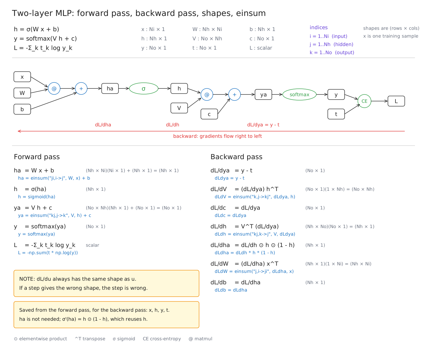
Reading it: the graph across the top is the forward direction, left to right, with rectangles for values, blue circles for the two arithmetic ops, and green for the nonlinearities and the loss. The red arrow underneath is the backward direction, with the three intermediate gradients marked at the points they’re computed. The two columns below pair each equation with its shape and its one line of code.
The code
Everything above, as a script that runs. The only thing worth flagging before the listing is how the column-vector convention from the math survives contact with numpy.
In the math, \(x\) is \(N_i \times 1\) and row vectors need an explicit \(x^\top\). In numpy the arrays are 1-D, shape (Ni,), with no stored orientation at all; numpy infers what you meant from the operation. So the transposes in the packed forms don’t map one-to-one onto .T in the code:
| Math | numpy | Why |
|---|---|---|
| \(W x\) | W @ x | matmul against a 1-D array contracts its last axis |
| \(V^\top (y-t)\) | V.T @ dLdya | a real transpose, because we contract \(V\)’s first index |
| \((y-t) \, h^\top\) | np.outer(dLdya, h) | @ between two 1-D arrays gives a scalar, not an outer product |
| \(\dfrac{\partial L}{\partial h} \odot h \odot (1-h)\) | dLdh * h * (1 - h) | * is elementwise |
The third row is the one that bites. dLdya @ h would give you a dot product, silently, with no shape error to warn you. Outer products have to be asked for by name.
import numpy as np

rng = np.random.default_rng(0)

Ni, Nh, No = 784, 500, 10                  # input, hidden, output

W = rng.normal(0, 0.01, (Nh, Ni));  b = np.zeros(Nh)
V = rng.normal(0, 0.01, (No, Nh));  c = np.zeros(No)

x = rng.normal(0, 1, Ni)                   # one training sample
t = np.zeros(No); t[3] = 1.0               # one-hot target, class 3


def sigmoid(z):
    return 1.0 / (1.0 + np.exp(-z))


def softmax(z):
    z = z - z.max()                        # subtract the max before exponentiating
    e = np.exp(z)
    return e / e.sum()


def forward(W, b, V, c):
    ha = W @ x + b                         # (Nh,)   eq (1)
    h  = sigmoid(ha)                       # (Nh,)   eq (2)
    ya = V @ h + c                         # (No,)   eq (3)
    y  = softmax(ya)                       # (No,)   eq (4)
    L  = -np.sum(t * np.log(y + 1e-12))    # scalar  eq (5)
    return h, y, L


h, y, L = forward(W, b, V, c)

# --- backward ---
dLdya = y - t                              # (No,)      eq (14)
dLdV  = np.outer(dLdya, h)                 # (No, Nh)   eq (15)
dLdc  = dLdya                              # (No,)      eq (16)
dLdh  = V.T @ dLdya                        # (Nh,)      eq (17)
dLdha = dLdh * h * (1.0 - h)               # (Nh,)      eq (18)
dLdW  = np.outer(dLdha, x)                 # (Nh, Ni)   eq (19)
dLdb  = dLdha                              # (Nh,)      eq (20)

# --- update ---
eta = 0.01
W -= eta * dLdW;  b -= eta * dLdb
V -= eta * dLdV;  c -= eta * dLdc
Two details in there that aren’t in the math. softmax subtracts the max before exponentiating; this changes nothing mathematically, since the constant cancels between numerator and denominator, but it keeps \(e^{z}\) from overflowing when the logits are large. And the loss adds 1e-12 inside the log, so a probability that has underflowed to exactly zero gives a large finite number instead of -inf. Neither affects the gradients, because we never differentiate through them; \(y - t\) was derived before either was introduced.
Checking it
Derivations look right far more often than they are right, so it’s worth making the machine check. The gradient of \(L\) with respect to one parameter entry is a plain scalar derivative, so we can approximate it with a central difference and compare:
\[\frac{\partial L}{\partial \theta} \approx \frac{L(\theta + \varepsilon) - L(\theta - \varepsilon)}{2\varepsilon}\]Central difference rather than \((L(\theta+\varepsilon) - L(\theta))/\varepsilon\) because its error shrinks like \(\varepsilon^2\) instead of \(\varepsilon\), which buys several digits for free.
def grad_check(name, P, dP, n=25, eps=1e-6):
    """Central finite difference on n random entries. Run before the update."""
    worst = 0.0
    for _ in range(n):
        idx = tuple(rng.integers(0, s) for s in P.shape)
        orig = P[idx]
        P[idx] = orig + eps;  Lp = forward(W, b, V, c)[2]
        P[idx] = orig - eps;  Lm = forward(W, b, V, c)[2]
        P[idx] = orig
        worst = max(worst, abs((Lp - Lm) / (2 * eps) - dP[idx]))
    print(f"dL/d{name}: max |analytic - numeric| = {worst:.2e}")


for name, P, dP in [("W", W, dLdW), ("b", b, dLdb), ("V", V, dLdV), ("c", c, dLdc)]:
    assert P.shape == dP.shape, f"{name}: {P.shape} vs {dP.shape}"
    grad_check(name, P, dP)
dL/dW: max |analytic - numeric| = 2.44e-10
dL/db: max |analytic - numeric| = 1.75e-10
dL/dV: max |analytic - numeric| = 2.72e-10
dL/dc: max |analytic - numeric| = 2.57e-10
Agreement to ten digits, which is about the floor for float64 at this \(\varepsilon\); the remaining error is roundoff in the two loss evaluations, not a flaw in the derivation. The assert on shapes is worth keeping too. It’s the convention-4 check turned into code, and it catches a transposed outer product instantly.
If you ever get a mismatch, the size of it tells you where to look. Off by a clean factor (2, or the batch size) means a missing or doubled sum. Off only for one parameter means one line is wrong. Off everywhere means the forward pass and the loss disagree about something.
Batching, in one index
Everything so far was a single sample. Real training uses a batch, and the whole change is one extra index.
Let \(n = 1 \dots N\) index the samples, and stack them as rows, so \(X\) is \(N \times N_i\) and row \(n\) is one input. The loss becomes the mean over the batch:
\[L = -\frac{1}{N} \sum_n \sum_k T_{nk} \log Y_{nk}\]Now look at what happens to the index \(n\) in each gradient, because there are exactly two cases:
Activations carry \(n\) through. Each sample has its own hidden vector, its own probabilities, its own intermediate gradients. Nothing is shared, so \(n\) just comes along:
\[\frac{\partial L}{\partial (H_a)_{nj}} = \frac{\partial L}{\partial H_{nj}} \, H_{nj}(1 - H_{nj})\]Parameter gradients sum \(n\) away. The same \(W\) is used by every sample, so every sample contributes a term, and the total derivative is the sum of those contributions. This is the many-routes chain rule again, with the routes now being the samples:
\[\frac{\partial L}{\partial W_{ji}} = \sum_n \frac{\partial L}{\partial (H_a)_{nj}} \, X_{ni}\]That sum over \(n\) is exactly what a matrix product does, which is why batching costs no extra code:
def softmax_rows(Z):                 # softmax along the last axis, per sample
    Z = Z - Z.max(axis=1, keepdims=True)
    E = np.exp(Z)
    return E / E.sum(axis=1, keepdims=True)


def forward(W, b, V, c):
    Ha = X @ W.T + b                 # (N, Nh)
    H  = sigmoid(Ha)                 # (N, Nh)
    Ya = H @ V.T + c                 # (N, No)
    Y  = softmax_rows(Ya)            # (N, No)
    return H, Y, -np.sum(T * np.log(Y + 1e-12)) / N


dLdYa = (Y - T) / N                  # (N, No)    the 1/N from the mean
dLdV  = dLdYa.T @ H                  # (No, Nh)   n summed away
dLdc  = dLdYa.sum(axis=0)            # (No,)      n summed away
dLdH  = dLdYa @ V                    # (N, Nh)    n carried through
dLdHa = dLdH * H * (1 - H)           # (N, Nh)    n carried through
dLdW  = dLdHa.T @ X                  # (Nh, Ni)   n summed away
dLdb  = dLdHa.sum(axis=0)            # (Nh,)      n summed away
Three things changed and nothing else. The outer products became matrix products, since dLdYa.T @ H sums over \(n\) where np.outer had nothing to sum. The bias gradients became explicit .sum(axis=0), because a bias is added to every row and therefore receives a contribution from every row. And the \(1/N\) from the mean rides along from the start, folded into dLdYa once rather than applied to each parameter gradient separately.
Note also that the parameter gradients keep exactly the shapes they had for a single sample; dLdW is still \(N_h \times N_i\) whichever batch size you use. That has to be true, since it’s still being subtracted from W. The batch dimension appears in the intermediates and is gone by the time you reach the parameters. Same gradient check applies, and it passes to the same ten digits.
Wrapping up
The thing I wanted out of writing this was the habit rather than the results. Derive on scalars where the chain rule is unambiguous, write the full sum and let the Kronecker deltas prune it, read off the packed form last, and check the shape at every line. Do that and the gradients fall out the same way every time, whether it’s a two-layer MLP or something with a lot more indices.
The results worth keeping in your head are small. Softmax with cross-entropy collapses to \(y - t\). A weight gradient is an outer product of the incoming gradient with the layer’s saved input. An input gradient is the transposed weight matrix times the incoming gradient, and the transpose is there because you’re contracting the first index. A bias gradient is the incoming gradient, unchanged. Elementwise activations have diagonal Jacobians, which is why they show up as * and not as matmuls. Those five facts cover every line of the backward pass above.
If you find a mistake anywhere in here, please let me know and I’ll fix it.