DeepSeek's Other Modules - Fine-Grained MoE, Hyper-Connections, Engram, and DSpark, From First Principles
Hello all. The previous post followed one number, the KV cache bytes per token, through four DeepSeek generations. This post covers everything in DeepSeek-V4.1-Flash that is not attention, and it needs a different organizing question: where do the parameters live, and which ones does a token actually touch? The model has 552B backbone parameters and another 196B in lookup tables, yet a decode token activates 16B and a prefill token 8B. Four mechanisms account for that gap and for how the activated ones are chosen and combined: a Mixture-of-Experts with 384 narrow experts per layer and a router that balances itself without a loss term; a residual stream carried as four copies, mixed at every sublayer by matrices constrained to a manifold; a 196B hashed n-gram memory that is read, not multiplied; and a speculative decoder that drafts five tokens per step and decides per request how many to verify.
Each gets the same treatment as before: the cost it attacks, the mechanism with tensor shapes, what it costs at serving time, and a diagram. Three short numpy checks are included where a claim can be tested on a laptop.
The plan:
- The parameter accounting: 552B, 196B, 16B, and 8B reconciled from config.json
- Fine-grained MoE and routing: DeepSeekMoE’s two ideas, bias-only balancing, the affinity function, hash-routed layers, per-modality biases, and the serving picture
- Hyper-connections and mHC: four residual streams, why unconstrained mixing explodes, the doubly stochastic fix, and the single-pass shift that halves memory traffic
- Engram: memory as a second sparsity axis, the lookup pipeline, the U-shaped allocation law, and V4.1’s two 98B tables
- DSpark: from MTP to block drafting, the Markov and confidence heads, and throughput-aware verification
- Takeaways, and a question bank
I’m assuming the LLM inference systems post for MoE basics, expert parallelism, and speculative decoding’s rejection rule, and the attention lineage post for the model’s attention and cache. Every number is from a linked paper, model card, or repository; config values come from each model’s config.json on Hugging Face, checked 2026-09-13; and quotes from DeepSeek’s reference inference code are from the inference/model.py and inference/engram.py files in the V4.1-Flash repository as of the same date.
Let’s get started.
The Parameter Accounting
Start with the arithmetic, because every section below is a piece of it. From config.json: hidden size 5120, 40 layers, 384 routed experts and 1 shared expert per layer with intermediate size 2304, 6 routed experts active per token.
One expert
An expert is a SwiGLU feed-forward network, three matrices: a gate projection and an up projection from 5120 to 2304, and a down projection back:
\[3 \times 5120 \times 2304 \approx 35.4\text{M parameters}\]That number is worth pausing on against the usual intuition. A dense transformer FFN is sized around \(d_{ff} = 4d\), and SwiGLU models usually take about \(\tfrac{8}{3}d\); the transformer block accounting post uses the \(4d\) convention. Here one expert is \(2304 / 5120 \approx 0.45d\) wide, narrower than a dense FFN by a lot. The width a token actually sees is seven experts, \(7 \times 2304 = 16{,}128 \approx 3.15d\), back in the familiar range; the width the model owns is \(385 \times 2304 \approx 173d\). That is fine-grained MoE in one line, and the next section is about why it is shaped this way.
The whole model
| Component | Computation | Parameters |
|---|---|---|
| Routed experts | \(384 \times 40 \times 35.4\text{M}\) | 543.6B |
| Shared experts | \(1 \times 40 \times 35.4\text{M}\) | 1.4B |
| Routers | \(40 \times 5120 \times 384\) | 0.08B |
| Everything else in the 552B backbone | by subtraction | about 6.9B |
| Engram tables (outside the backbone) | \((384{,}006{,}168 + 384{,}016{,}682) \times 256\) | 196.6B |
The 6.9B remainder holds 40 layers of attention (query and output low-rank projections, the 512-wide latent path, the indexers and compressors), the embedding table and untied output head at \(129{,}280 \times 5120 \approx 0.66\text{B}\) each, the hyper-connection coefficient projections, norms, and whatever share of the vision encoder the report counts as backbone; the report does not itemize it. The Engram row is exact: the two row counts are in the config and each row is 256 channels, and the vLLM recipe’s memory table lists the tables at 196.6B parameters and 188.8 GiB in FP8.
Per token
| Phase | Layers run | Experts per layer | MoE parameters touched | Plus attention and dense | Total |
|---|---|---|---|---|---|
| Decode | 40 | 6 routed + 1 shared | \(40 \times 7 \times 35.4\text{M} = 9.9\text{B}\) | about 6B | 16B |
| Prefill | 20 (the encoder) | 6 routed + 1 shared | \(20 \times 7 \times 35.4\text{M} = 5.0\text{B}\) | about 3B | 8B |
The 16B and 8B match the model card within rounding. The prefill row is the causal encoder-decoder from the attention post: a prompt token runs only the bottom 20 layers, so it touches half the experts. Not counted: the embedding lookup, which is a gather rather than a matmul; the Engram lookups, which are also gathers; and the DSpark drafter, which runs only when speculative decoding is on. The reports do not state exactly which of these the 16B includes, so treat the table as reproducing the number, not defining it.
References
- DeepSeek-V4.1-Flash config.json, model card, tech report section 4.2.1
- vLLM recipe memory table
- Transformer block accounting post
Fine-Grained MoE and Routing
The cost: a dense FFN spends every parameter on every token
A dense feed-forward layer multiplies each token by all of its weights. Capacity and compute are the same number. Mixture-of-Experts breaks the tie: keep \(N\) expert FFNs, and let a router send each token to \(K\) of them, so capacity scales with \(N\) while compute scales with \(K\). In the conventional form (DeepSeekMoE paper, equations 3 to 5), the output is a gated sum over the selected experts, with gates \(g_{i,t}\) equal to the softmax affinity \(s_{i,t} = \mathrm{Softmax}_i(u_t^{\top} e_i)\) between the token and a learned centroid \(e_i\) for the top-\(K\) experts and zero elsewhere. The inference post covers the serving consequences: all \(N\) experts must be resident, routing becomes all-to-all traffic, and skew across experts is the throughput risk.
DeepSeekMoE’s two ideas
The January 2024 DeepSeekMoE paper (Dai et al.) changed the shape of the experts rather than the routing, with two moves.
Fine-grained segmentation. “We segment each expert FFN into \(m\) smaller experts by reducing the FFN intermediate hidden dimension to \(1/m\) times its original size. Since each expert becomes smaller, in response, we also increase the number of activated experts to \(m\) times to keep the same computation cost” (section 3.1). Same parameters, same FLOPs, \(mN\) experts with \(mK\) active. The argument is combinatorial: with 16 experts and top-2 there are \(\binom{16}{2} = 120\) ways to combine experts for a token; split each into 4 and route top-8 among 64, and there are \(\binom{64}{8} = 4{,}426{,}165{,}368\). For V4.1-Flash’s top-6 of 384 the count is about \(4.3 \times 10^{12}\) (my arithmetic). More combinations means each expert can specialize more narrowly and the router can assemble knowledge more precisely.
Shared expert isolation. “We further isolate \(K_s\) experts to serve as shared experts. Regardless of the router module, each token will be deterministically assigned to these shared experts” (section 3.2), and the routed count is reduced by \(K_s\) to hold compute constant. The shared expert absorbs whatever every token needs, so the routed experts do not each have to relearn it.
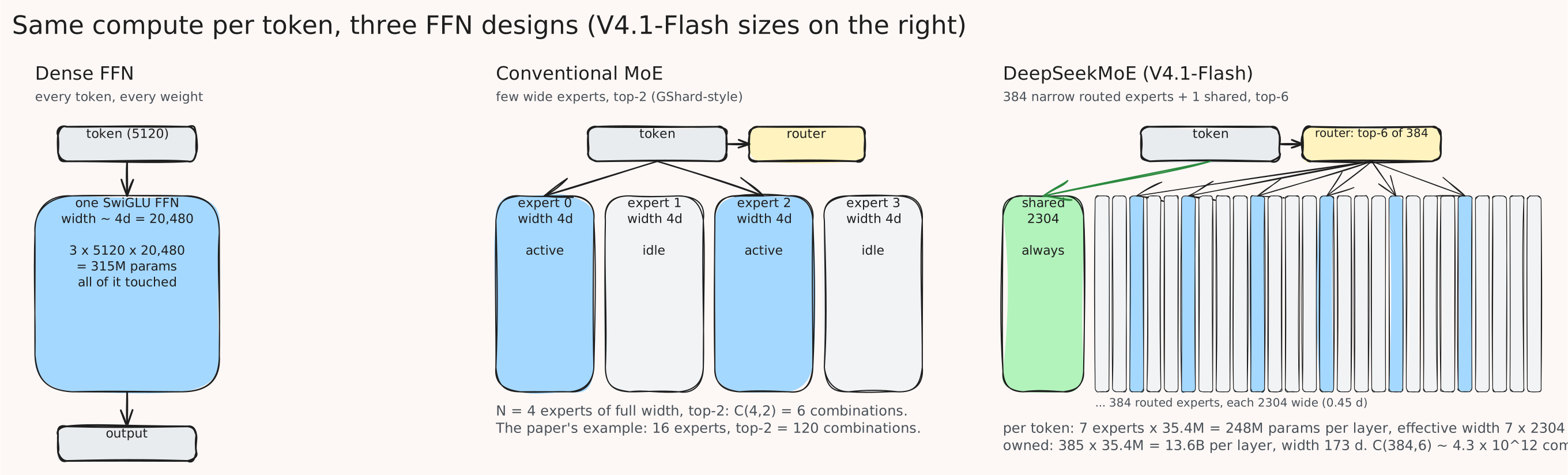
The paper’s headline evidence: DeepSeekMoE 16B, with 2 shared and 64 routed experts at a quarter of a standard FFN’s width and 6 active, matched LLaMA2 7B “with only 39.6% of computations” (section 5.2.2). The lineage since then has kept the shape and scaled the counts:
| Model | Routed / shared | Active routed | Expert width | Hidden | Source |
|---|---|---|---|---|---|
| DeepSeekMoE 16B | 64 / 2 | 6 | 1408 | 2048 | config |
| DeepSeek-V2 | 160 / 2 | 6 | 1536 | 5120 | V2 paper section 3.1.2 |
| DeepSeek-V3 | 256 / 1 | 8 | 2048 | 7168 | V3 report section 4.2 |
| DeepSeek-V4-Flash | 256 / 1 | 6 | 2048 | 4096 | V4 report section 4.2.1 |
| DeepSeek-V4-Pro | 384 / 1 | 6 | 3072 | 7168 | same |
| DeepSeek-V4.1-Flash | 384 / 1 | 6 | 2304 | 5120 | V4.1 report section 4.2.1 |
Balancing without a loss
Routers collapse: left alone, a few experts win most tokens, the rest starve, and both quality and parallel efficiency suffer. The classic fix is an auxiliary balance loss that penalizes uneven load, and DeepSeekMoE used one at the expert level and another at the device level (section 3.3). The problem, stated in the Auxiliary-Loss-Free Load Balancing paper (Wang et al., 2024): “a large auxiliary loss will introduce non-negligible interference gradients into training and thus impair the model performance.” Too small a coefficient and routing collapses; too large and the model gets worse (their Figure 2).
The loss-free rule replaces the gradient with a bias that touches only selection (equation 3):
\[g_{i,t} = \begin{cases} s_{i,t} & \text{if } s_{i,t} + b_i \in \mathrm{Topk}(\{s_{j,t} + b_j\}, K) \\ 0 & \text{otherwise} \end{cases}\]The bias \(b_i\) decides which experts are picked; the gate value that scales the expert’s output is the unbiased affinity \(s_{i,t}\). After each training step, count tokens per expert, and nudge: “\(b_i = b_i + u \cdot \mathrm{sign}(e_i)\)” where \(e_i\) is the shortfall of expert \(i\) against the mean load (Algorithm 1). Overloaded experts get a lower bias and win fewer ties next step. Nothing flows into the model’s gradients. The update uses historical load rather than the current sequence’s, because “utilizing the load information of the current sequence will break the causal constraint of language modeling.” On their 3B model, perplexity went from 7.97 to 7.92 and the maximum load violation from 0.52 to 0.04 (Table 2).
DeepSeek-V3 adopted this as its main balancer with update speed \(\gamma = 0.001\), plus a “complementary sequence-wise auxiliary loss” at a tiny coefficient of 0.0001 “to prevent extreme imbalance within any single sequence” (V3 report, section 2.1.2 and 4.2). Balancing per batch rather than per sequence is itself a feature: the report’s ablation argues batch-wise balance “does not enforce in-domain balance on each sequence,” which lets experts specialize by domain.
The affinity function, and V4.1’s per-modality biases
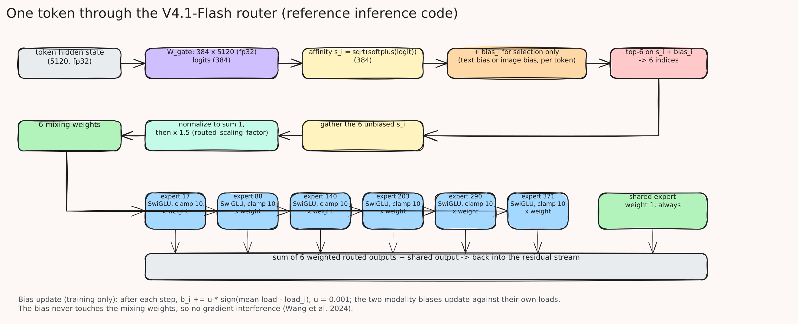
Three more routing changes arrive across the generations, and the reference router shows all of them at once.
| Generation | Affinity \(s_{i,t}\) | Gate normalization | Placement limit | Source |
|---|---|---|---|---|
| V2 | softmax over experts | none | device-limited | V2 paper |
| V3 | sigmoid | renormalize over the selected \(K\) | at most 4 nodes per token | V3 report section 2.1.2 |
| V4 | \(\sqrt{\mathrm{Softplus}(\cdot)}\) | renormalize | limit removed | V4 report section 2.1 |
| V4.1 | \(\sqrt{\mathrm{Softplus}(\cdot)}\) | renormalize, then scale by 1.5 | none | config, reference code |
The V3 report explains the sigmoid: it “uses the sigmoid function to compute the affinity scores, and applies a normalization among all selected affinity scores.” The V4 report states the change to \(\sqrt{\mathrm{Softplus}}\) but gives no reason for it. The node limit in V3 existed so a token’s experts sat on at most 4 of the 8 nodes hosting them, bounding cross-node traffic; V4 “remove[s] the constraint on the number of routing target nodes, and carefully redesign[s] the parallelism strategy.” The scale factor, routed_scaling_factor in every config since V3, is never named in a report; V2 mentions “additional scaling factors at the width bottlenecks … to ensure stable training,” and the code shows where it applies.
V4.1 adds the multimodal twist. Image tokens and text tokens “may induce different expert-routing preferences,” so balancing their combined load can hide a modality-specific imbalance. The fix keeps two bias vectors per layer, one per modality, updated independently against each modality’s own load (V4.1 report, section 2.1.1). The router from the reference inference/model.py, as of 2026-09-13:
scores = linear(x.float(), self.weight.float()) / self.gate_temp
scores = F.softplus(scores).sqrt()                      # the V4 affinity
bias = self.bias
if image_mask is not None and self.bias_vl is not None:
    bias = torch.where(image_mask.unsqueeze(-1), self.bias_vl, bias)   # per-modality bias
# the bias picks experts but does not scale them: weights come from the raw scores
indices = (scores + bias).topk(self.topk, dim=-1)[1]
weights = scores.gather(1, indices)
if self.norm_topk_prob and self.topk > 1:
    weights /= weights.sum(dim=-1, keepdim=True) + 1e-20
weights *= self.route_scale                             # 1.5 in config.json
Every line above maps to a paper: the affinity is V4’s, the bias-for-selection-only is the loss-free rule, the modality switch is V4.1’s, the renormalization is V3’s, and the scale is the unexplained constant. The router runs in fp32, which matters when 384 scores compete for 6 slots.
Two more details: hash-routed layers and the clamp
V4 replaced the dense first layers that V3 kept with MoE layers using hash routing for the first three: the expert is chosen by a fixed function of the token id, not by the router (Hash Layers, Roller et al., 2021: “the hash function is fixed in advance, and in this way, our routing mechanism requires no training and has no adjustable parameters”). The V4 reference code looks the expert up in a [vocab_size, active] table and still computes learned gate scores for the mixing weights. V4.1’s config has no hash-layer key and its router has no hash branch, so V4.1 appears to have dropped them; no report says so, so that is an inference from config and code.
The SwiGLU clamp is a training-stability device that ships with the weights. V4’s report: “we clamped the linear component of SwiGLU to the range of \([-10, 10]\), while capping the upper bound of the gate component at 10,” which “effectively eliminates outliers” (section 4.2.3). The expert code applies exactly that, up branch clamped both sides, gate branch capped from above, with the routing weight multiplying the intermediate before the down projection. V4.1 keeps it at threshold 10 (swiglu_limit).
How many experts a batch touches
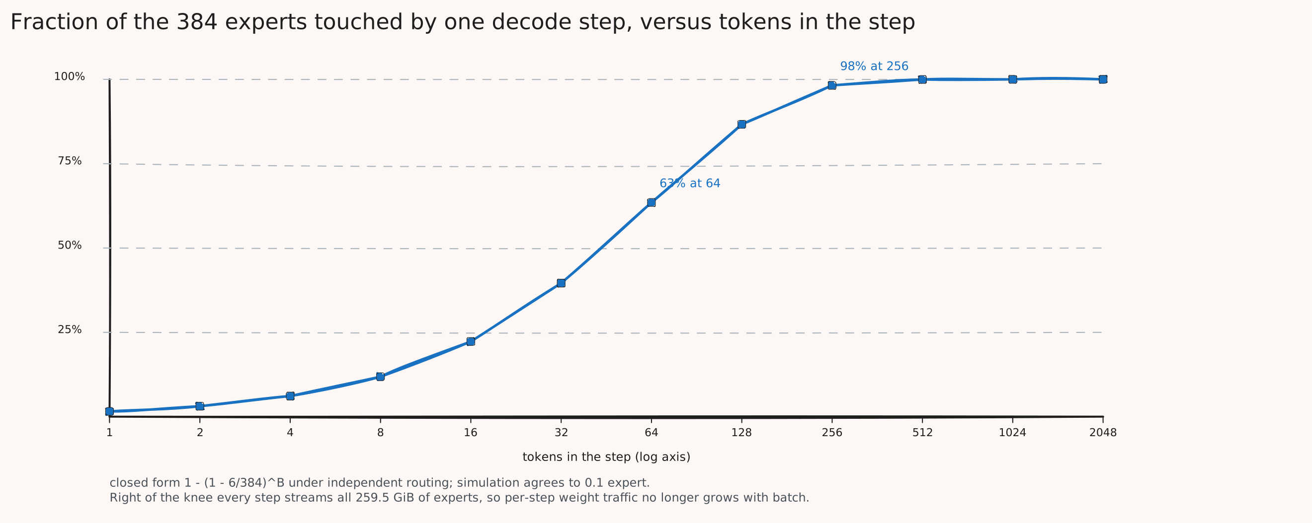
For serving, the question is not which expert a token picks but how many distinct experts a step reads, because every expert read is a weight stream from HBM. With top-6 of 384 and routing treated as independent draws, the expected number touched by a batch of \(B\) tokens is
\[384 \times \big(1 - (1 - 6/384)^B\big)\]A short simulation confirms the closed form (numpy 2.4.1, 2026-09-13):
import numpy as np
rng = np.random.default_rng(0)
E, k = 384, 6
for B in (1, 8, 64, 256, 1024):
    touched = []
    for _ in range(200):                        # 200 random batches
        picks = np.array([rng.choice(E, k, replace=False) for _ in range(B)])
        touched.append(len(np.unique(picks)))
    closed = E * (1 - (1 - k / E) ** B)
    print(f"B={B:5d}: experts touched, simulated {np.mean(touched):6.1f}  closed form {closed:6.1f}  "
          f"= {100*closed/E:5.1f}% of {E}")
B=    1: experts touched, simulated    6.0  closed form    6.0  =   1.6% of 384
B=    8: experts touched, simulated   45.7  closed form   45.5  =  11.8% of 384
B=   64: experts touched, simulated  243.8  closed form  243.8  =  63.5% of 384
B=  256: experts touched, simulated  377.1  closed form  377.2  =  98.2% of 384
B= 1024: experts touched, simulated  384.0  closed form  384.0  = 100.0% of 384
By a few hundred tokens per step, a step reads essentially all 259.5 GiB of experts, and the per-step weight traffic stops depending on batch size. Real routing is not uniform, which is what balancing is for, but the shape of the curve is what decides where decode stops being weight-bound. The briefing post uses this curve for the B300 arithmetic.
The serving picture
Three facts from the papers frame how these layers are served. First, the experts are the model: 259.5 GiB of the checkpoint’s 476 GiB, so expert parallelism shards them across GPUs and every MoE layer becomes an all-to-all dispatch and combine, the topology the inference post describes. Second, skew is handled at deployment, not only in training. DeepSeek-V3’s production layout duplicated hot experts: “the high-load experts are detected based on statistics collected during the online deployment and are adjusted periodically (e.g., every 10 minutes),” with 32 redundant experts in the prefill pool, and the decode pool treated the shared expert as a routed one that every token picks (V3 report, section 3.4). vLLM’s EPLB is the same idea. Third, DeepSeek fuses the whole layer: DeepGEMM’s Mega-MoE “fuses and overlaps EP dispatch, linear 1 and linear 2 (FP8xFP4 or FP8xFP8), SwiGLU, and EP combine into a single mega-kernel,” and its Mega-Gate fuses the router matmul with top-k and takes the per-modality bias and the physical placement map as arguments, so redundant-expert routing happens inside the gate kernel. The V4.1 report’s “15 kernels in prefill, 11 in decode” per layer counts these as one each.
References
- DeepSeekMoE: Towards Ultimate Expert Specialization in Mixture-of-Experts Language Models, Dai et al. 2024, sections 3 and 5
- Auxiliary-Loss-Free Load Balancing Strategy for Mixture-of-Experts, Wang et al. 2024
- DeepSeek-V2, DeepSeek-V3 Technical Report sections 2.1.2, 3.4, 4.2, 4.5; DeepSeek-V4 sections 2.1 and 4.2.3; V4.1 tech report sections 2.1.1 and 3.2
- Hash Layers For Large Sparse Models, Roller et al. 2021
- V4.1-Flash reference inference code, V4-Flash reference code, DeepGEMM
Hyper-Connections and mHC
The cost: one residual stream, fixed connection strengths
Every transformer since the original carries a single residual stream. In the pre-norm form (Xiong et al., 2020), each sublayer computes \(x_{l+1} = x_l + F(\mathrm{LN}(x_l))\): the input passes through unchanged and the sublayer’s output is added with weight one. Unrolled, \(x_L = x_l + \sum_i F(\ldots)\), and the identity term is what makes deep stacks trainable (He et al., 2016). The Hyper-Connections paper (Zhu et al., ByteDance, 2024) argues that this fixes something it should not: “residual connections, including both Pre-Norm and Post-Norm variants, predefine the strength of connections between the output and input within a layer,” and the two variants sit at opposite ends of a “seesaw” between representation collapse (pre-norm: adjacent layers’ features become nearly identical) and vanishing gradients (post-norm).
Hyper-connections: n streams and three mixing maps
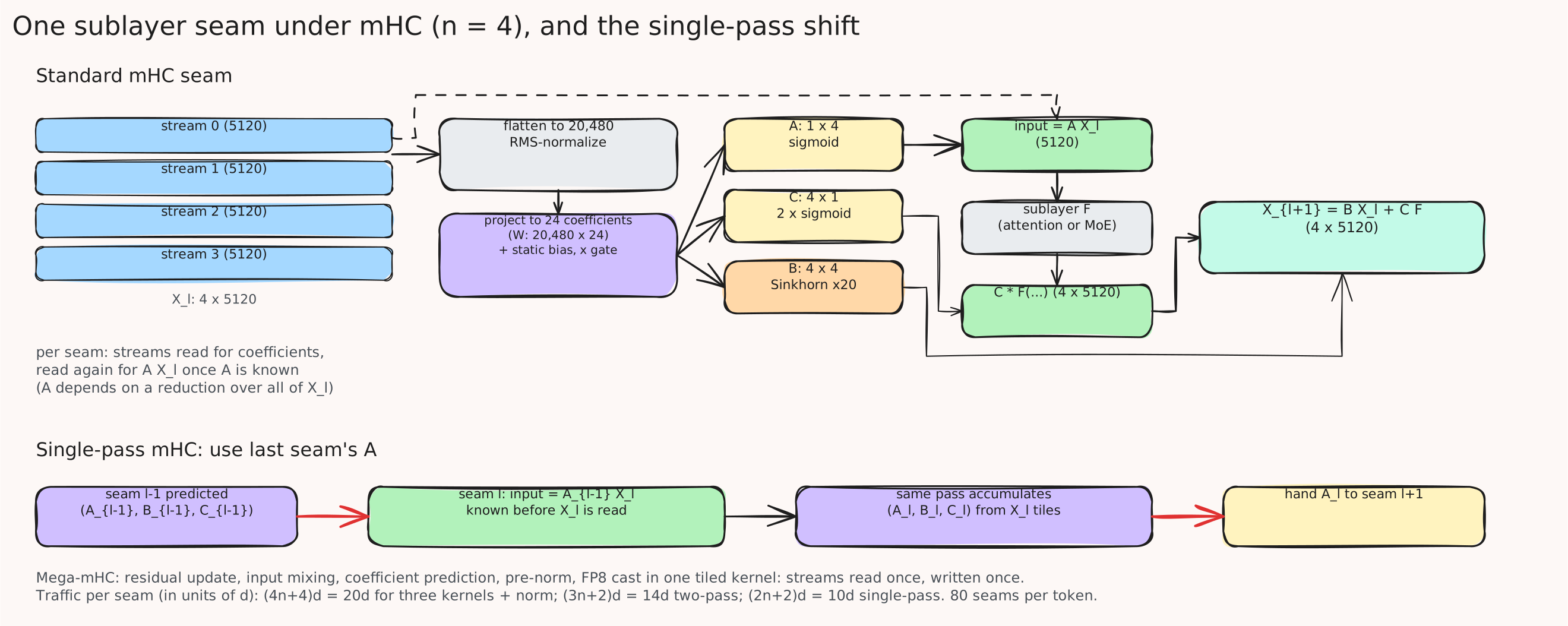
The proposal widens the residual stream to \(n\) copies, \(X_l \in \mathbb{R}^{n \times d}\), and makes the connections learnable. In the notation the DeepSeek-V4 report uses (section 2.2, equation 1):
\[X_{l+1} = B_l X_l + C_l\, F_l(A_l X_l)\]with three coefficient sets per sublayer: an input map \(A_l \in \mathbb{R}^{1 \times n}\) that collapses the \(n\) streams into one \(d\)-wide sublayer input, an output map \(C_l \in \mathbb{R}^{n \times 1}\) that writes the sublayer’s output back into the streams, and a residual map \(B_l \in \mathbb{R}^{n \times n}\) that mixes the streams among themselves. With \(n = 1\) and all three fixed at 1 this is the plain residual. The coefficients are dynamic: predicted per token from the stream itself by a small projection, plus static biases and a learned gate initialized near zero so that training starts from the residual connection. Each layer has two such modules, one around attention and one around the FFN, so there are \(2L\) seams per token.
The reported gain was real: on the ByteDance OLMoE-1B-7B run, dynamic hyper-connections at \(n = 4\) “converges 1.8 times faster compared to the baseline,” at a parameter cost under 0.04% and a FLOP cost around 0.2% (Appendix B). The memory cost is the catch, and it comes in two forms the paper does not fully price: \(n\) times the activation storage, and \(n\) times the memory traffic at every seam.
Why unconstrained mixing explodes
DeepSeek’s mHC paper (Xie et al., 2026) found the failure when scaling. Unroll the residual map across layers and the identity term of the plain residual becomes a product of learned matrices, \(\prod_i B_{L-i}\). “The composite mapping … fails to preserve the global mean of the features. This discrepancy leads to unbounded signal amplification or attenuation, resulting in instability during large-scale training” (section 1). Measured on a 27B model, the maximum gain of that composite map through the network “yields extreme values with peaks of 3000,” and the training loss surged around step 12k, correlated with a gradient-norm spike (Figures 2 and 3).

The fix: keep \(B_l\) doubly stochastic
mHC constrains the residual map to the set of doubly stochastic matrices, non-negative with every row and every column summing to 1 (equation 6):
\[B_l \in \mathcal{M} = \{ M \in \mathbb{R}^{n \times n} \mid M \mathbf{1}_n = \mathbf{1}_n,\ \mathbf{1}_n^{\top} M = \mathbf{1}_n^{\top},\ M \geq 0 \}\]Three properties follow and the paper names each (section 4.1). The spectral norm of such a matrix is at most 1, so the map is non-expansive and cannot amplify. The set is closed under multiplication, so the composite across any number of layers is still doubly stochastic, still non-expansive. And the set is the Birkhoff polytope, the convex hull of permutation matrices, so each mixing step is a convex combination of stream permutations: the feature mean across streams is conserved exactly. At \(n = 1\) the only doubly stochastic matrix is the scalar 1, and the plain residual is recovered.
The projection onto the set is the Sinkhorn-Knopp algorithm: exponentiate the raw coefficients so every entry is positive, then alternately normalize rows and columns to sum to 1. Twenty iterations in every DeepSeek model since (hc_sinkhorn_iters in the config). The input and output maps get simpler constraints, \(A_l = \sigma(\tilde A_l)\) and \(C_l = 2\sigma(\tilde C_l)\), non-negative so that “positive and negative coefficients” cannot cancel a signal. The coefficients themselves come from one projection of the flattened, RMS-normalized stream: \(\mathrm{vec}(X_l) \in \mathbb{R}^{nd}\) times a matrix with \(n^2 + 2n = 24\) output columns at \(n = 4\), plus static biases and gates initialized at 0.01. The V4 report notes this 24-wide matmul is small enough that a deterministic split-K reduction had to be written for it (section 3.3).
Check it in numpy
Twenty iterations on a random 4-by-4, and the three properties:
import numpy as np
rng = np.random.default_rng(0)
n = 4
B_tilde = rng.standard_normal((n, n))          # the raw residual-mixing coefficients for one token
M = np.exp(B_tilde)                            # step 0: make every entry positive
for t in range(20):                            # 20 Sinkhorn-Knopp iterations, as in the config
    M = M / M.sum(axis=1, keepdims=True)       # rows sum to 1
    M = M / M.sum(axis=0, keepdims=True)       # columns sum to 1
    if t in (0, 4, 19):
        print(f"iter {t+1:2d}: max |row sum - 1| = {np.abs(M.sum(1)-1).max():.1e}, "
              f"max |col sum - 1| = {np.abs(M.sum(0)-1).max():.1e}")
print("spectral norm      :", np.linalg.norm(M, 2).round(6))
P = np.linalg.matrix_power(M, 80)              # 80 seams of the same matrix, the worst case
print("after 80 products  : spectral norm", np.linalg.norm(P, 2).round(6),
      " row sums", P.sum(1).round(6))
x = rng.standard_normal((n, 8))
print("mean over streams  : before", x.mean(0).round(3)[:4], " after", (M @ x).mean(0).round(3)[:4])
iter  1: max |row sum - 1| = 8.2e-02, max |col sum - 1| = 2.2e-16
iter  5: max |row sum - 1| = 1.9e-05, max |col sum - 1| = 1.1e-16
iter 20: max |row sum - 1| = 2.2e-16, max |col sum - 1| = 0.0e+00
spectral norm      : 1.0
after 80 products  : spectral norm 1.0  row sums [1. 1. 1. 1.]
mean over streams  : before [-0.265  0.458  0.307  0.314]  after [-0.265  0.458  0.307  0.314]
Row and column sums converge to machine precision well before 20 iterations, the spectral norm is exactly 1, eighty products of the map are still doubly stochastic, and the mean over the four streams is untouched to the printed precision. That last line is the “conserved feature mean” claim. The paper’s result on the 27B model: the composite gain’s maximum drops from about 3000 to about 1.6, the loss surge disappears, and the final loss is 0.021 below the baseline, with the whole thing costing 6.7% of training wall time at \(n = 4\) (sections 4.3 and 5).
Single-pass mHC: halving the traffic
V4 trained with mHC; V4.1’s contribution is to make it cheap to serve (V4.1 report, section 2.4.1). The accounting is in activation traffic per seam, in units of \(d\). The ideal seam reads the previous streams and the previous sublayer output, \((n+1)d\), and writes the new streams and the new sublayer input, \((n+1)d\): a floor of \((2n+2)d\). V4’s implementation needed three dependent kernels, residual update, coefficient prediction, input mixing, plus the pre-norm, reading and writing \((4n+4)d\), “twice the lower bound.” Two of the three can share one pass over the streams, because the residual update needs no reduction across the hidden dimension and each tile can feed the coefficient accumulators as it goes. The input mixing cannot join, because \(A_l\) depends on a reduction over all tiles of \(X_l\), so it needs a second read: \((3n+2)d\).
The single-pass idea removes the dependency by moving it one seam back (equation 6):
\[X_{l+1} = B_l X_l + C_l\, F_l(A_{l-1} X_l), \qquad (A_l, B_l, C_l) = H(X_l)\]The input map applied at seam \(l\) is the one predicted at seam \(l - 1\), so it is known before \(X_l\) is read, and every tile of \(X_l\) can be mixed into the sublayer input and fed to the coefficient accumulators in the same pass. “Empirically, this shift incurs negligible performance degradation.” Pre-training keeps the multi-kernel form, since the shift only changes which coefficients a seam applies. Deployment fuses residual update, input mixing, coefficient prediction, pre-norm, and the FP8 cast into one Mega-mHC kernel, at the \((2n+2)d\) floor, “halving the activation memory traffic of our original implementation.” In the reference code the hand-off is a returned tensor: each sublayer’s seam returns the input map for the next, and the attention seam uses the one the previous layer’s FFN produced.
For V4.1-Flash, \(n = 4\) and \(d = 5120\), so the floor is \(10d = 51{,}200\) elements per seam and there are \(2 \times 40 = 80\) seams per token: about 4.1M elements, 7.8 MiB in bf16, of pure residual traffic per token, against 15.6 MiB under V4’s scheme. My arithmetic, from the report’s coefficients and the config.
The serving cost is launches, not bytes
The traffic accounting explains why DeepSeek fused the kernel. The one public trace of this model in vLLM, an AMD RFC on MI355X, explains why it matters more than the bytes suggest: “a decode step issues 14,020 kernel launches, and 85% of each layer’s 350 launches are attributable to the mHC block, bookkeeping on a 4x4 matrix.” Their breakdown puts 162 launches per layer in the Sinkhorn loop and 122 in the pre and post mixing with an eager RMSNorm, against 24 for the entire MoE layer and 6 for attention. A 4-by-4 matrix normalized 20 times per seam, 80 seams per token, as unfused PyTorch ops, is thousands of launches for microseconds of arithmetic. The RFC’s fix routes the seam to a fused kernel and takes it “from 141 to 4 launches per seam.” That is the same lesson as the fused Mega-mHC kernel, arrived at from the other side: mHC’s cost at inference is entirely about how few kernels it can be.
References
- Deep Residual Learning for Image Recognition, He et al. 2016; On Layer Normalization in the Transformer Architecture, Xiong et al. 2020
- Hyper-Connections, Zhu et al. 2024, sections 1 to 3 and Appendix B
- mHC: Manifold-Constrained Hyper-Connections, Xie et al. 2026, sections 1, 3, 4, 5
- DeepSeek-V4 sections 2.2, 3.3, 3.4.2; V4.1 tech report section 2.4.1; V4.1 reference code
- vLLM RFC #56506, DeepSeek-V4.1-Flash performance on ROCm
Engram
The cost: reconstructing a lookup table with matmuls
MoE scales capacity by choosing which weights to multiply. The Engram paper (Cheng et al., DeepSeek, 2026) argues that a second kind of sparsity is missing: “Transformers lack a native primitive for knowledge lookup, forcing them to inefficiently simulate retrieval through computation.” Much of language is “local, static, and highly stereotyped,” named entities and fixed phrases, and resolving a multi-token entity “requires consuming multiple early layers of attention and feed-forward networks,” which “essentially amounts to an expensive runtime reconstruction of a static lookup table.” The paper’s illustration, borrowed from interpretability work, is “Diana, Princess of Wales” assembling piece by piece across layers 1 to 6 of an LLM.
The proposal is conditional memory: a module that retrieves a static embedding by the identity of the last few tokens, in \(O(1)\), and lets the network’s depth go to reasoning instead. Conditional computation (MoE) picks parameters to multiply; conditional memory picks parameters to read.
The lookup pipeline
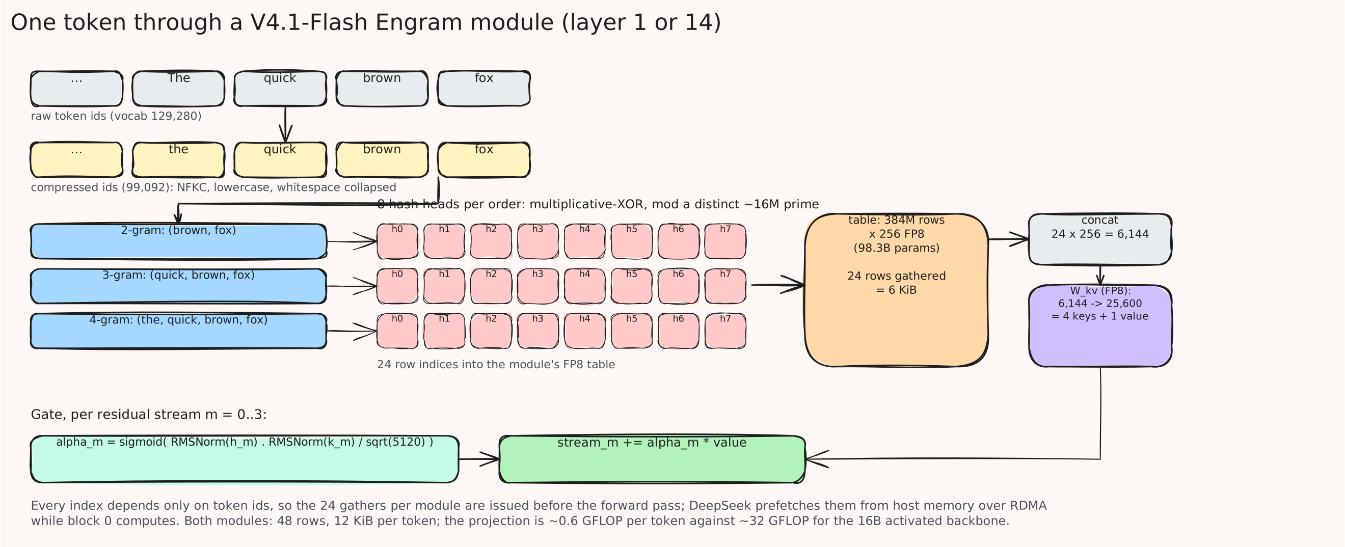
Engram is an n-gram embedding table modernized in three ways (paper, section 2).
Tokenizer compression. Raw token ids over-distinguish: The, ` the, and THE are different tokens carrying the same knowledge. A precomputed surjection maps each token to a canonical id "based on normalized textual equivalence (using NFKC, lowercasing, etc.)," which "achieves a 23% reduction in the effective vocabulary size for a 128k tokenizer." V4.1's config confirms the ratio: 129,280 raw ids compress to 99,092, a 23.4% reduction (engram_compressed_vocab_size`). Suffix n-grams are then formed over compressed ids.
Multi-head hashing. Each n-gram order \(n\) has \(K\) hash heads, and each head \(k\) maps the n-gram into its own table of prime size \(M_{n,k}\) (equation 1):
\[z_{t,n,k} = \phi_{n,k}(g_{t,n}), \qquad e_{t,n,k} = E_{n,k}[z_{t,n,k}]\]with \(\phi\) “a lightweight multiplicative-XOR hash.” Several heads with different prime moduli mean that two n-grams colliding in one table almost surely differ in the others, so the concatenation over orders and heads (equation 2) is nearly unique even though each table is far smaller than the number of possible n-grams. The reference code draws one odd 64-bit multiplier per look-back position, XORs the multiplied ids together, and takes the result modulo each head’s prime; the primes are chosen once, in order, never reused across the whole model.
Context-aware gating. A retrieved embedding can be wrong for the context (“bank” near a river). The current hidden state \(h_t\), which has already been through attention, is used as a query against a key projected from the memory, and the sigmoid of their normalized dot product scales a value projection (equations 3 and 4):
\[k_t = W_K e_t, \quad v_t = W_V e_t, \quad \alpha_t = \sigma\!\left(\frac{\mathrm{RMSNorm}(h_t)^{\top} \mathrm{RMSNorm}(k_t)}{\sqrt{d}}\right), \quad \tilde v_t = \alpha_t v_t\]“If the retrieved memory \(e_t\) contradicts the current context \(h_t\), the gate \(\alpha_t\) tends toward zero.” The gated value is added to the residual stream, \(H \leftarrow H + \tilde V\), before the layer’s attention. With hyper-connections the value projection is shared and each of the four streams gets its own key projection and gate, so the projections fuse into one FP8 matmul (section 2.4). The paper also had a short depthwise convolution after the gate; V4.1 drops it.
Check it in Python
The compression and hashing steps are pure string and integer operations, so a small demo shows the property that matters: case and spacing variants of the same phrase land in the same rows.
import unicodedata
def compress(tok):                               # tokenizer compression: NFKC, strip accents, lowercase, collapse whitespace
    s = unicodedata.normalize("NFKC", tok)
    s = "".join(c for c in unicodedata.normalize("NFD", s) if not unicodedata.combining(c))
    return " ".join(s.lower().split()) or " "
vocab = sorted({compress(t) for t in ["The", " the", "THE", "thé", "cat", " Cat", "sat"]})
cid = {c: i + 1 for i, c in enumerate(vocab)}   # compressed ids; 0 is reserved for padding
MULT = [0x9E3779B97F4A7C15, 0xC2B2AE3D27D4EB4F, 0x165667B19E3779F9]   # one odd multiplier per look-back
PRIMES = [16000057, 16000073, 16000093]        # one prime-sized table per hash head
def ngram_rows(ids, n):                          # multiplicative-XOR hash of the last n compressed ids
    ids = [0] * (n - 1) + ids
    rows = []
    for t in range(n - 1, len(ids)):
        h = ids[t] * MULT[0]
        for i in range(1, n):
            h ^= ids[t - i] * MULT[i]
        rows.append([h % p for p in PRIMES])
    return rows
for text in [["The", "cat", "sat"], [" the", " Cat", "sat"], ["THE", "cat", "sat"]]:
    ids = [cid[compress(t)] for t in text]
    print(f"{str(text):28s} -> compressed ids {ids} -> 3-gram rows at 'sat': {ngram_rows(ids, 3)[-1]}")
['The', 'cat', 'sat']        -> compressed ids [3, 1, 2] -> 3-gram rows at 'sat': [12747208, 14583992, 11240134]
[' the', ' Cat', 'sat']      -> compressed ids [3, 1, 2] -> 3-gram rows at 'sat': [12747208, 14583992, 11240134]
['THE', 'cat', 'sat']        -> compressed ids [3, 1, 2] -> 3-gram rows at 'sat': [12747208, 14583992, 11240134]
Seven raw tokens become three compressed ids, and all three spellings of the phrase hash to the same three rows, one per head. The multipliers, the 16-million-sized primes, and the XOR structure mirror the reference engram.py; the normalization is a simplification of its rules, which also handle partial UTF-8 byte tokens.
What the paper found
The paper’s central experiment holds total and active parameters fixed and moves a fraction of the inactive budget from experts to memory. The result is “a consistent U-shaped relationship between validation loss and the allocation ratio”: pure MoE is not the optimum, reallocating roughly a fifth to a quarter of the sparse parameter budget to Engram “yields the best performance,” and at the 10B scale the loss improves from 1.7248 to 1.7109 (section 3.1). Memory size alone follows a power law over two orders of magnitude of table size (section 3.2).

At 27B parameters and 262B tokens, replacing 17 of 72 experts with 5.7B parameters of memory raised MMLU from 57.4 to 60.4, BBH from 50.9 to 55.9, and multi-query needle-in-a-haystack retrieval at 32K context from 84.2 to 97.0 (Tables 1 and 2). Ablating the module at inference drops factual-recall benchmarks to 29 to 44 percent of their score while reading-comprehension tasks keep 81 to 93 percent (section 6.3), which is the cleanest evidence that what the tables hold is facts. And placement matters: a single module does best at layer 2, “early enough to replace the backbone’s bottom-layer local aggregation” but after one round of attention so the gate has a contextualized query (section 6.2).
V4.1’s two tables, reconciled
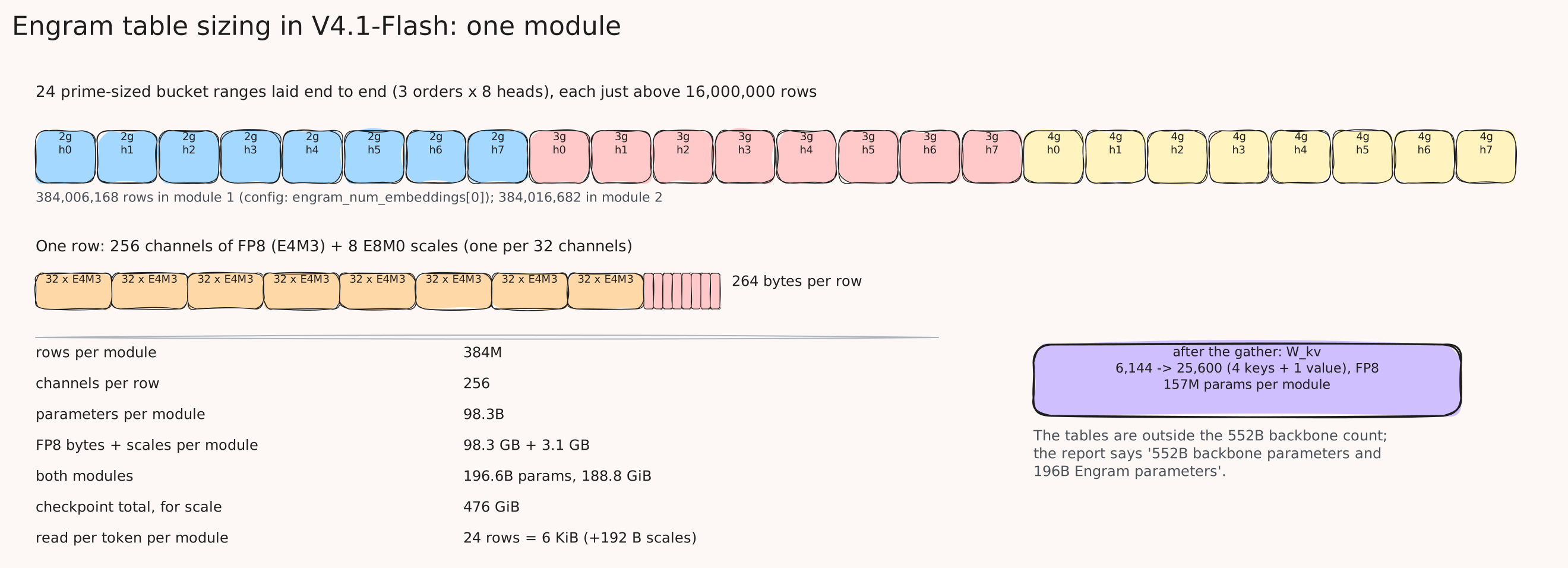
The V4.1 instantiation (report, section 2.4.2): two modules at layers 1 and 14, “196B Engram parameters evenly across two modules. Each module uses N-gram orders {2, 3, 4}, with 8 hash heads and a total embedding dimension of 2048 per order. Each head indexes a table of approximately 16M entries, with table sizes chosen to be distinct primes.” Tables and projections are FP8.
The config makes this exact. Three orders times eight heads is 24 bucket ranges per module, each a prime just above 16,000,000, and the reference code’s prime generator, rerun, gives 24 primes starting at 16,000,057 whose sum is 384,006,168, the first entry of engram_num_embeddings; the second module’s 24 primes sum to 384,016,682, the second entry. Each row is one head’s 256-channel embedding (engram_head_dim), so:
In FP8 with one E8M0 scale per 32 channels, 8 scale bytes per row, that is 98.3 GB plus 3.1 GB per module, 188.8 GiB for both, which is the recipe’s figure. The projection after the lookup is a single matrix from \(24 \times 256 = 6{,}144\) inputs to \(5 \times 5120 = 25{,}600\) outputs, four keys and one value, 157M parameters per module.
Serving cost: gathers, not FLOPs
Per token per module, 24 rows of 256 FP8 bytes is 6 KiB plus 192 bytes of scales; both modules, 12 KiB. The projection is about 0.6 GFLOP per token for both modules against roughly 32 GFLOP for the 16B activated backbone. Bandwidth and arithmetic are both negligible. What is not negligible is where 189 GiB of tables sit and how long a random 256-byte read takes to arrive from there.
The design answer is that the addresses are known early. “Engram lookup indices depend solely on the input token sequence,” so “deterministic addressing enables embeddings to be prefetched from host memory via background RDMA transfers, with prefetching for the first module overlapping computation in the first Transformer block” (report, sections 2.4.2 and 3.1.3). The Engram paper measured the same idea on H800s: a 100B-parameter table kept entirely in host DRAM cost at most 2.8% of throughput on a dense 8B backbone, because “the effective communication volume per step scales with the number of activated slots rather than the total embedding table size” (section 6.4, Table 4). The paper also sketches a tiered layout, hot rows in HBM, the long tail on NVMe, since n-gram frequencies are Zipfian. During RL rollouts DeepSeek keeps the tables in GPU memory instead, “to avoid out-of-memory failures caused by host memory fragmentation.” Where a serving engine puts them, and whether it prefetches, is the decision the briefing post spends a section on.
References
- Conditional Memory via Scalable Lookup: A New Axis of Sparsity for Large Language Models, Cheng et al. 2026, sections 2, 3, 4, 6; code
- V4.1 tech report sections 2.4.2, 2.5, 3.1.3; config.json; reference engram.py
- vLLM recipe memory table
DSpark
The cost: one token per weight read
Decode reads the model’s active weights once per step and produces one token per sequence. The inference post’s decode-floor section works out why that makes the step memory-bound and how speculative decoding attacks it: a cheap drafter proposes several tokens, the target verifies them in one forward pass, and a rejection rule keeps the longest correct prefix while leaving the output distribution exactly the target’s (Leviathan et al., 2023). With acceptance rate \(\alpha\) and \(\gamma\) drafted tokens, the expected tokens per step is \((1 - \alpha^{\gamma+1})/(1 - \alpha)\). Every design question after that is about the drafter: how it proposes, how much it costs, and how many of its tokens to bother verifying.
Lineage: MTP, and why production stayed at one token
DeepSeek-V3 trained with a multi-token prediction objective: one extra Transformer block per prediction depth that takes the main model’s hidden state and the next token’s embedding and predicts the token after that, “keep[ing] the complete causal chain at each prediction depth” (V3 report, section 2.2). The depth was 1, the goal was better training, and the module was repurposed for speculative decoding at an acceptance rate of “85% and 90%” for “1.8 times TPS” (section 5.4.3). V4 kept it unchanged. The DSpark paper (Cheng et al., DeepSeek, 2026) explains why production never went past one drafted token: “deploying a static multi-token drafter (e.g., MTP-3/5) strictly degrades aggregate throughput under high concurrency due to excessive verification overhead” (section 5.4). At low load the GPU has idle compute to verify long drafts; at high load every rejected draft token is compute stolen from real tokens. A fixed draft length is wrong at one end or the other.
Block drafting: five positions in one pass
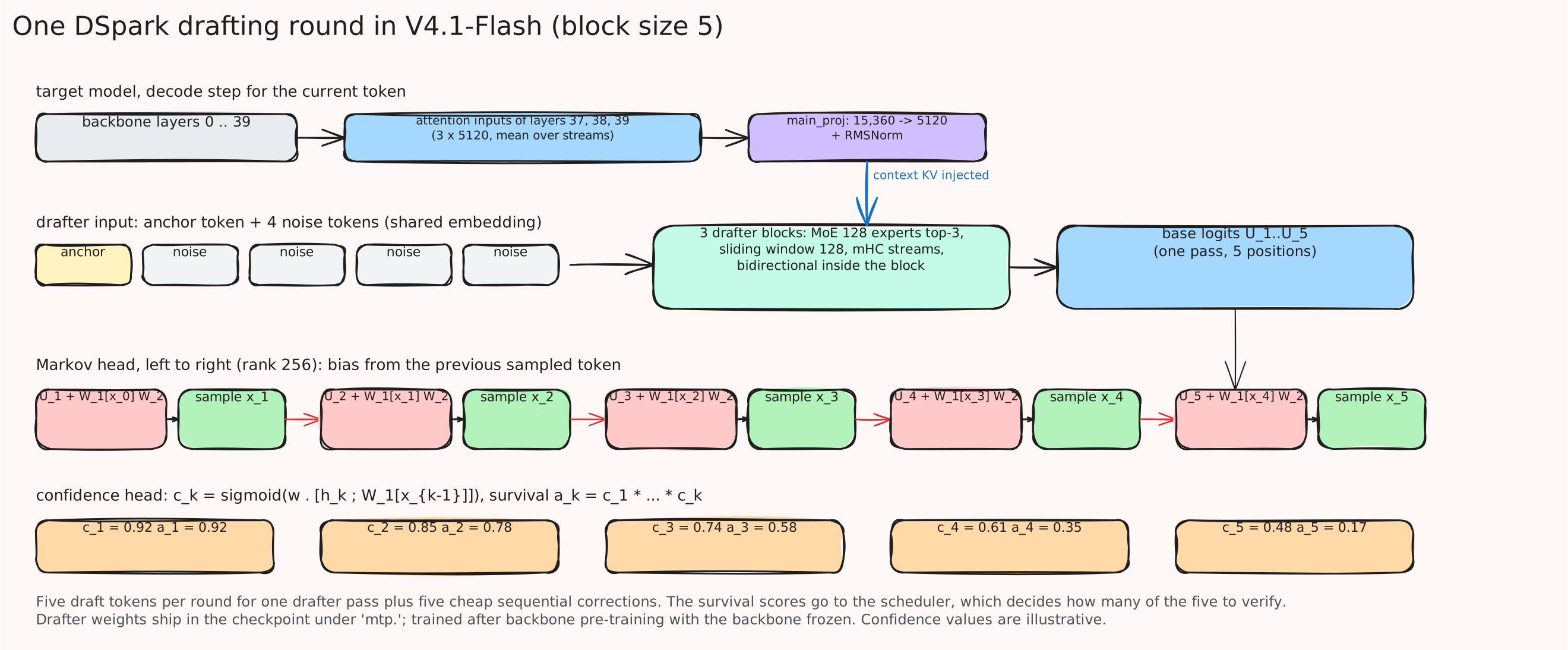
DSpark’s drafter is semi-autoregressive. Its backbone is DFlash, a block-diffusion drafter: feed the anchor token plus \(\gamma - 1\) placeholder tokens through a few Transformer blocks that attend bidirectionally within the block and to context features injected from the target model, and get logits for all \(\gamma\) positions from one forward pass. The V4.1 drafter (config and report, section 2.4.3) is three Transformer blocks with a 128-token sliding window, each an MoE of 128 routed experts with 3 active, reading the attention inputs of backbone layers 37 to 39 through one projection; the block size is 5, and the placeholder is a dedicated noise token (dspark_noise_token_id). The drafter’s weights ship in the checkpoint under the mtp prefix, and it was trained after backbone pre-training with the backbone frozen, then kept in step through post-training “without propagating gradients from the DSpark objective into the backbone.”
A purely parallel draft has a weakness: position 3’s logits do not know what position 2 sampled, so the block can be internally inconsistent. DSpark adds a cheap sequential correction. Given base logits \(U_k\) for each position, the draft distribution is (paper, equation 4)
\[p_k(v \mid x_0, x_{<k}) \propto \exp\big(U_k(v) + B_k(x_0, x_{<k}, v)\big)\]and the default Markov head makes the bias depend only on the previous drafted token through a rank-256 factorization, \(B(x_{k-1}, \cdot) = W_1[x_{k-1}]\, W_2\) (equation 5): a 129,280-by-256 embedding and its transpose-shaped output map, 33M parameters each. Sampling the block left to right is then five tiny matrix-vector products after one drafter pass. The paper’s example: once position 1 samples “of”, the head “boosts ‘course’ and suppresses ‘problem’ at position 2.” On Qwen3-4B the Markov head lifts accepted length per round from DFlash’s 5.40 to 6.11 on GSM8K and from 2.96 to 3.54 on Alpaca chat (Table 1).
The confidence head and the scheduler
The second idea is to decide, per request and per step, how much of the block to verify. A confidence head predicts for each position “the conditional probability that the draft token at position \(k\) will survive target verification, given that all preceding tokens in the block have been accepted” (equation 7, a sigmoid over the drafter’s hidden state and the Markov embedding of the previous token). Its training target is the analytical acceptance rate, one minus half the L1 distance between the draft and target distributions (equation 8), and a per-position temperature scaling brings its calibration error to about 1%. Multiplying confidences along a draft gives each position a survival probability, the chance that everything up to it is accepted.
The scheduler (paper, section 3.2.2, Algorithm 1) then treats verification as a budget problem across the whole batch. Every (request, position) slot has a survival score; sort all slots by it; add slots one at a time, extending that request’s verified prefix, and track the expected accepted tokens per second, \(\tau \times \mathrm{SPS}(B)\), where \(B\) is the total tokens in the step and \(\mathrm{SPS}\) is the engine’s steps per second at that batch size, “profiled once during engine initialization and stored as a lightweight cost table.” Stop the first time adding a slot lowers the product. Because survival is non-increasing along a draft, the greedy walk is exact for a fixed budget, and because it breaks at the first drop it never uses information from later slots, which keeps the decision causal. The effect is that a confident request’s fifth token can be verified while a doubtful request’s second is not, and the average verified length falls smoothly as load rises: roughly four to six tokens per request at moderate concurrency, down toward MTP-1’s fixed 2 as the engine saturates (Figure 8).
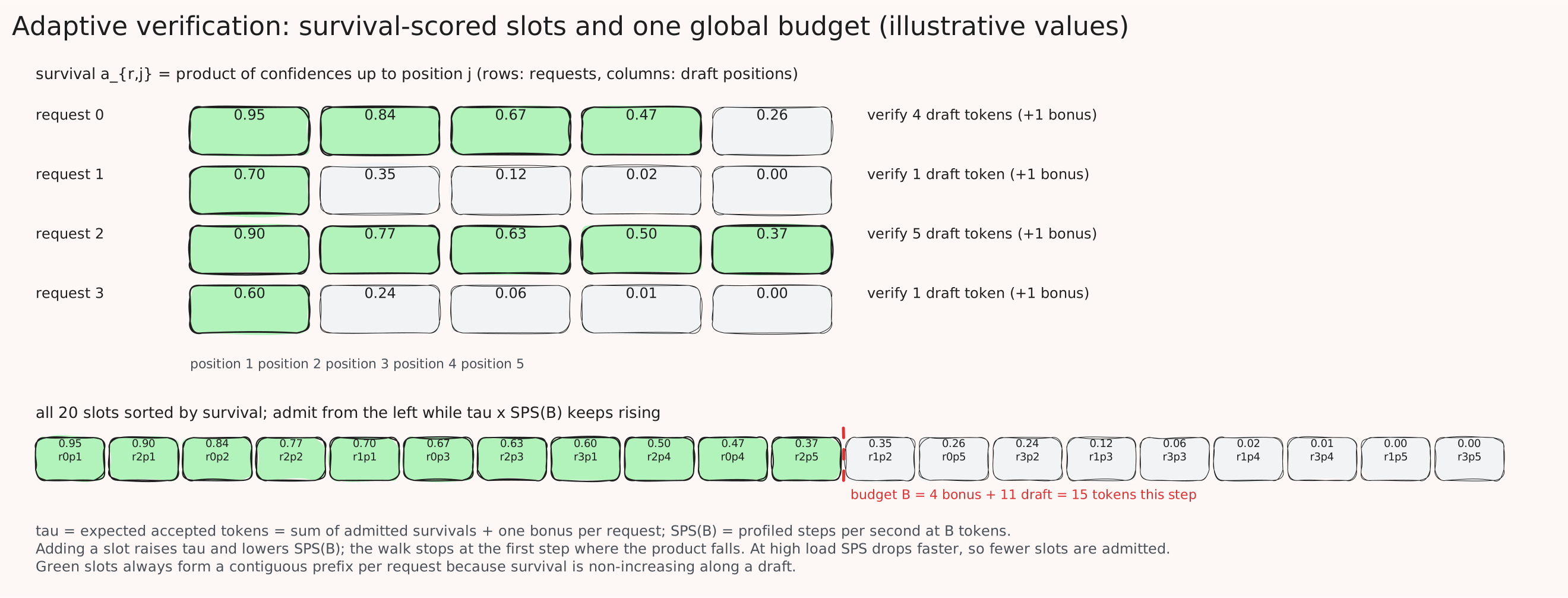
Two production details from the paper’s section 5.2 matter for reading engine behavior. The scheduler runs asynchronously with CUDA graphs, so the budget is sized from confidence values “from two steps prior,” while the per-request ordering uses current values; and the profiled step-time curve is “jagged” in practice, staircase-shaped inside CUDA-graph capture sizes, so early stopping on the raw curve was replaced by the delayed budget.
Verification
The paper verifies with standard rejection sampling at temperature 1, accepting draft token \(x_k\) with probability \(\min(1, p_t(x_k)/p_d(x_k))\) and stopping at the first rejection, so “the acceptance rule preserves the target distribution exactly.” vLLM’s recipe for V4.1 sets two extra knobs the paper does not name: draft_sample_method: probabilistic, meaning the draft samples from its distribution and the full draft probabilities enter the ratio test, and rejection_sample_method: block, which is block verification (Sun et al., 2024), a lossless variant that verifies the whole draft jointly and is never worse than token-by-token. vLLM’s adaptive verification is the scheduler above: “every (request, position) draft slot is scored by its survival probability … and the highest-scoring slots are admitted until a global budget is spent,” with the budget chosen by an argmax over a cumulative sum against a profiled cost table, and it “is only supported for DSpark with a confidence head.”
What it bought
On DeepSeek’s own serving stack, DSpark with block size 5 replaced MTP-1 two weeks after the V4 preview and, at an 80 tokens-per-second-per-user target, “improves aggregate throughput by 51%” on V4-Flash and 52% on V4-Pro, with per-user generation speed up by 60 to 85 percent at matched throughput (section 5.4, Figure 7). The same numbers do not exist for V4.1-Flash; the report gives none, and the vLLM adaptive-verification post that ran V4-Pro on 8x B300 reports its sweep as a plot without printed values. What the vLLM post does state is the motivating fact: on V4-Pro “the last drafted token of a 7-token block survives less than 10% of the time, against more than 70% for the first,” which is exactly the decay the scheduler exists to price. In SGLang’s V4.1 recipe DSpark is on in the low-latency configuration and off in the high-throughput one, “at large batch the fixed step cost stops paying for itself,” which is the static version of the same trade the scheduler makes dynamically.
References
- DSpark: Confidence-Scheduled Speculative Decoding with Semi-Autoregressive Generation, Cheng et al. 2026, sections 2, 3, 4, 5
- DFlash: Block Diffusion for Flash Speculative Decoding, Chen et al. 2026; Fast Inference from Transformers via Speculative Decoding, Leviathan et al. 2023; Block Verification Accelerates Speculative Decoding, Sun et al. 2024
- DeepSeek-V3 Technical Report sections 2.2 and 5.4.3; V4.1 tech report section 2.4.3; V4.1 config.json
- vLLM adaptive verification doc, vLLM DSpark adaptive verification post, vLLM recipe, SGLang cookbook
- LLM inference systems post, speculative decoding section
Takeaways
- The 552B is almost entirely experts: 543.6B routed, 1.4B shared, and about 6.9B for everything else. A decode token touches 7 experts per layer, 9.9B of expert weights plus about 6B of attention and dense weights, 16B; a prefill token runs half the layers, 8B.
- Fine-grained MoE trades width for choice. Experts 0.45d wide, seven active for 3.15d of effective width, and trillions of ways to combine them; a shared expert holds what every token needs.
- Balance is a bias, not a loss. The router adds a per-expert bias for selection only, nudged by sign after each step from historical load, so no gradient interferes with the language objective. V4.1 keeps one bias per modality.
- Four residual streams, mixed by a doubly stochastic matrix. Unconstrained mixing compounds to gains in the thousands; Sinkhorn-Knopp projection makes every mixing step non-expansive and mean-preserving, and 80 such seams per token cost launches far more than bytes.
- Single-pass mHC halves residual traffic by shifting one coefficient back one seam, which lets a single fused kernel read the streams once.
- Engram is memory as sparsity. Compressed ids, hashed n-grams, 24 rows of 256 FP8 channels per module gated by the current context; 196B parameters read at 12 KiB per token, prefetched because the addresses are known before the forward pass.
- DSpark drafts five tokens in one pass and verifies as many as the load allows. A Markov head fixes intra-block consistency, a confidence head prices each position, and a throughput-aware scheduler turns verification into a batch-wide budget.
Test Yourself
Try each from memory before reading the answer.
1. How many parameters does one V4.1-Flash expert have, and how did you get there? Three matrices of \(5120 \times 2304\): gate, up, and down. About 35.4M.
2. Why is an expert narrower than a dense FFN, and what width does a token actually see? Fine-grained segmentation splits the FFN budget into many narrow experts so the router has more combinations to choose from. One expert is 2304 wide, about 0.45d; a token sees 6 routed plus 1 shared, 16,128 channels, about 3.15d.
3. What does the load-balancing bias touch, and what does it not touch? It is added to the affinities only for the top-k selection. The gate value that scales an expert’s output is the unbiased affinity. The bias moves by a fixed step in the direction that corrects each expert’s historical load.
4. Name the affinity function of V3, V4, and V4.1, and the normalization applied after selection. V3: sigmoid. V4 and V4.1: square root of softplus. In all three, the selected affinities are renormalized to sum to 1, then scaled by the configured routing scale factor.
5. What does a hyper-connection’s residual map do, and what goes wrong without a constraint? It mixes the \(n\) residual streams with a learned \(n \times n\) matrix at every sublayer seam. Unconstrained, the product of those matrices across layers does not preserve the feature mean and its gain can grow to the thousands, destabilizing training.
6. State the doubly stochastic constraint and the three properties it buys. Non-negative entries with every row and column summing to 1. Spectral norm at most 1, so no amplification; closure under multiplication, so the composite stays bounded; and membership in the Birkhoff polytope, so each mix is a convex combination of permutations and the stream mean is conserved.
7. What does single-pass mHC change, and why does that allow one kernel? The input map applied at seam \(l\) is the one predicted at seam \(l-1\). The sublayer input no longer waits on a full reduction over the current streams, so residual update, input mixing, coefficient prediction, and pre-norm can run in one tiled pass with the streams read once and written once.
8. How many seams does a V4.1 token pass through, and why did the AMD trace blame them for most kernel launches? Eighty: one before attention and one before the FFN in each of 40 layers. Unfused, each seam runs 20 Sinkhorn iterations on a 4-by-4 matrix as separate ops, hundreds of launches per layer for microseconds of work.
9. Walk a token through an Engram module. Compress the token id, form the 2-, 3-, and 4-gram over compressed ids, hash each with 8 heads into prime-sized bucket ranges, gather 24 rows of 256 FP8 channels, concatenate to 6,144, project to four keys and one value, gate the value by each residual stream’s normalized dot product with its key, add to the stream.
10. Why can Engram tables live in host memory without stalling decode? The addresses depend only on the token ids, so the gathers are issued before the forward pass and the first module’s rows arrive while the first Transformer block computes; the volume is 12 KiB per token, so bandwidth is not the constraint.
11. Why did DeepSeek’s production stay at one MTP token before DSpark? A fixed multi-token draft wastes compute on rejected tokens at high concurrency, where the GPU is no longer memory-bound, and degrades aggregate throughput. A fixed length is wrong at one end of the load range or the other.
12. What do the Markov head and the confidence head each fix? The Markov head adds a bias from the previous drafted token to each position’s base logits so the block is internally consistent. The confidence head predicts each position’s chance of surviving verification, which the scheduler multiplies into survival scores.
13. How does the scheduler pick how many draft tokens to verify? Sort every (request, position) slot by survival probability across the batch, add slots in that order while expected accepted tokens times the profiled steps-per-second at the resulting batch size keeps rising, and stop at the first decrease. Each request ends up with a contiguous prefix whose length depends on its confidence and the current load.
Wrapping up
Four modules, and the same shape of idea under each: decide what a token touches, and make the decision cheap. The router chooses seven of 385 experts with a bias that costs nothing to train and an fp32 matmul that costs almost nothing to run. The hyper-connections choose how four residual streams mix, with a constraint that turns a stability problem into a projection, and a one-seam shift that turns three kernels into one. Engram chooses 24 rows out of 768 million by hashing the last four tokens, before the forward pass has even started. DSpark chooses how many drafted tokens each request gets to verify, by a sort and a profiled cost table, every step.
Taken with the attention post, this is the whole of DeepSeek-V4.1-Flash as an architecture: what is cached, what is multiplied, what is read, and what is guessed. Each of those is a lever the serving stack can pull or leave alone, and the briefing post is about which ones vLLM pulls today.
If you find a mistake anywhere in here, please let me know and I’ll fix it.