Large-Scale LLM Training Systems - How and Why
Hello all. This post is the training-side companion to the LLM inference systems post: how the systems that train large language models across thousands of GPUs are put together, and why they are shaped the way they are.
The inference post had one organizing fact, that generating a token is cheap on arithmetic and expensive on memory traffic, and everything in a serving engine followed from it. Training has its own organizing fact, and it is a different one. A training step does three times the arithmetic of a forward pass, holds an optimizer’s worth of state for every parameter, and keeps every intermediate activation alive until the backward pass consumes it. So training is not bandwidth-bound the way decode is; it is capacity-bound first and communication-bound second. The model’s state does not fit on one GPU, so it has to be split, and once it is split, every step has to move bytes between GPUs to stitch it back together. Nearly every technique below, mixed precision, activation recomputation, ZeRO, tensor and pipeline parallelism, is an answer to one of two questions: how do we make the state smaller, and how do we hide the communication that splitting it creates.
The angle is general rather than framework-specific. Ideas are anchored in the papers and official documents that introduced them, Megatron-LM, ZeRO, GPipe, PipeDream, the FSDP and DDP papers, the FP8 and mixed precision papers, and the Llama 3 report, which is the running real-world example because it publishes its actual parallelism configuration, its measured utilization, and its failure statistics. Every number quoted here was checked against a linked source, and each major section ends with its references. Arithmetic derived from those numbers is worked out in the open so you can check it.
The plan:
- Why training is a different shape from inference, and where the \(6N\) comes from
- The numbers that drive everything: the hardware, the bytes per parameter, and activation memory
- Mixed precision: fp16, bf16, loss scaling, FP8
- Activation recomputation, and why it is a throughput optimization
- Communication primitives: the collectives, the ring algorithm, and the cost model
- Data parallelism: DDP, gradient accumulation, ZeRO, FSDP, and offloading
- Tensor parallelism: column-then-row splits and what the all-reduces cost
- Sequence, context, and expert parallelism
- Pipeline parallelism: microbatches, the bubble, and the schedules
- Composing them: 3D and 4D parallelism, and how a real run is laid out
- MFU and HFU: the utilization numbers and how to compute them in both directions
- What breaks at scale
- Takeaways
- Test yourself: a question bank over everything above
I’m assuming you’re comfortable with what a transformer is and with backpropagation at the level of the MLP forward and backward post. This is a long one, but the sections build in order, and the question bank at the end is there to check what stuck.
Let’s get started.
Why Training Is a Different Shape
Start with a side-by-side, because the two workloads run the same model and could hardly be more different:
| Inference (decode) | Training | |
|---|---|---|
| FLOPs per token | \(\approx 2N\) | \(\approx 6N\) |
| What fills memory | weights and the KV cache | weights, gradients, optimizer state, and saved activations |
| First bottleneck | HBM bandwidth (the weight read per step) | HBM capacity (the state does not fit) |
| Second bottleneck | latency of the small collectives under TP | interconnect bandwidth for the sharded state |
| Batch | as large as the latency budget allows | as large as memory allows, then gradient accumulation |
| Arithmetic intensity | roughly the batch size, low | high; big batched GEMMs in both directions |
| Utilization metric | fraction of bandwidth, tokens/s per replica | MFU, fraction of peak FLOP/s |
Two rows carry the rest of the post: the FLOPs row and the memory row.
Where the \(6N\) comes from
\(N\) is the parameter count excluding the embedding table. A forward pass costs about \(2N\) FLOPs per token, because a token passing through a linear layer with \(k \times n\) weights is a \(1 \times k\) row times a \(k \times n\) matrix, which is \(2kn\) FLOPs, two per parameter, one multiply and one add. Summed over every weight matrix in the model that is \(2N\). This is Kaplan et al., Eq. 2.2, which also carries an attention term, \(2 \, n_{layer} \, n_{ctx} \, d_{model}\), that grows with context and stays small until contexts get long. The transformer block accounting post has the op-by-op ledger.
The backward pass costs about twice the forward. Kaplan states it as an approximation, and the reason is worth having exactly, because it is the answer to “why 6 and not 4”. Take one linear layer \(u = A z\) with \(A\) of shape \(m \times n\), and let \(g = \partial L / \partial u\) be the gradient arriving from downstream. The backward pass has to produce two things:
\[\frac{\partial L}{\partial A} = g \, z^\top \qquad (m \times n), \qquad\qquad \frac{\partial L}{\partial z} = A^\top g \qquad (n \times 1)\]The first is the weight gradient, an outer product of the incoming gradient with the saved input. The second is the input gradient, the transposed weight times the incoming gradient, which is what gets handed to the layer below. (Both are derived as equations (11) and (12) of the MLP post.) Over a batch of tokens each of these is a matrix multiply with exactly the same \(m\), \(n\), \(k\) dimensions as the forward multiply, so each costs the same \(2\) FLOPs per parameter per token that the forward did. Two of them make \(4N\), and \(2N + 4N = 6N\).
So the shape of a training step is three matmuls per weight matrix where inference has one, and one of the three, the weight gradient, has no counterpart in inference at all. Keep that outer product in mind; it is the reason the backward pass needs the forward pass’s inputs, which is the reason activations have to be saved, which is where most of the memory goes.
The organizing idea
Inference is a bandwidth problem: decode reads every weight once per token and does almost nothing with it. Training is a memory and communication problem: the state per parameter is many times the weight itself, the activations scale with the batch, none of it fits on one device, and every way of splitting it across devices creates traffic. The rest of this post is that sentence, unpacked.
References
- Scaling Laws for Neural Language Models - Kaplan et al.
- A Simple MLP - Forward Pass, Backward Pass, and Every Derivative (the outer-product and transposed-matmul shapes)
- Transformer Block FLOPs and Parameters Calculations
The Numbers That Drive Everything
Before any mechanism, the numbers. Three of them: the hardware and its bandwidth ladder, the bytes a training run holds per parameter, and the bytes it holds per token of activation. Every later section quotes these. All figures were checked against the linked sources.
The hardware
The H100 SXM is the reference GPU, since Llama 3 was trained on 80 GB H100s in 8-GPU NVLink servers (Llama 3 paper, Section 3.3.1); NVIDIA’s own DGX H100 supplies the node-level numbers:
| H100 SXM | Source | |
|---|---|---|
| Memory | 80 GB HBM3 | H100 page |
| HBM bandwidth | 3.35 TB/s | H100 page |
| BF16 tensor core, dense | \(\approx 989\) TFLOPS (1,979 “with sparsity”) | H100 page, footnote |
| FP8 tensor core, dense | \(\approx 1{,}979\) TFLOPS | same |
| NVLink (4th gen, 18 links) | 900 GB/s total, 450 GB/s per direction | Hopper in-depth |
| PCIe Gen5 x16 | 128 GB/s total, 64 GB/s per direction | Hopper in-depth |
| Node | 8 GPUs, all-to-all over NVSwitch | DGX H100 guide |
| Network | 8 ConnectX-7 at up to 400 Gb/s InfiniBand, one per GPU | DGX H100 guide |
Two reading notes. The marketing TFLOPS assume 2:4 structured sparsity; the datasheet footnote says the dense numbers are half, and dense is what training does. And NVLink’s 900 GB/s is the sum of both directions across 18 links at 25 GB/s each way, so a one-way stream sees 450 GB/s; the same applies to PCIe’s 128 GB/s.
What matters for parallelism is not any one number but the ladder they form, in bandwidth available to one GPU in one direction:
| Link | One-way bandwidth per GPU | Relative to HBM |
|---|---|---|
| HBM3 (on-package) | 3,350 GB/s | 1 |
| NVLink (within the node) | 450 GB/s | about 1/7 |
| InfiniBand NDR (across nodes) | 400 Gb/s = 50 GB/s | about 1/67 |
| PCIe Gen5 (to the host) | 64 GB/s | about 1/52 |
Each rung down is roughly an order of magnitude. Every parallelism decision in this post is, in the end, a decision about which traffic goes on which rung, and the rule that falls out is stated in the composition section: the chattiest split goes on the fastest link.
The models
The Llama 3 family is the running example, because its architecture table is public (Llama 3 paper, Table 3) and its training configuration is too:
| 8B | 70B | 405B | |
|---|---|---|---|
| Layers \(L\) | 32 | 80 | 126 |
| \(d_{model}\) (the paper’s \(h\)) | 4096 | 8192 | 16384 |
| Attention heads \(a\) | 32 | 64 | 128 |
| KV heads | 8 | 8 | 8 |
| head_dim | 128 | 128 | 128 |
| FFN dim | 14336 | 28672 | 53248 |
I’ll use the nominal parameter counts, \(8 \times 10^9\), \(70 \times 10^9\), \(405 \times 10^9\), in the arithmetic.
Bytes per parameter: the number that decides every design
A model trained in mixed precision with Adam holds, for every parameter (ZeRO paper, Section 3.1):
| Component | Precision | Bytes | Why it exists |
|---|---|---|---|
| Weights | bf16 or fp16 | 2 | what the forward and backward pass actually multiply with |
| Gradients | bf16 or fp16 | 2 | the \(g z^\top\) from the previous section |
| Master weights | fp32 | 4 | the authoritative copy the optimizer updates (next subsection) |
| Adam first moment \(m\) | fp32 | 4 | running mean of the gradient |
| Adam second moment \(v\) | fp32 | 4 | running mean of the squared gradient |
| Total | 16 |
The ZeRO paper calls the optimizer’s share \(K = 12\) bytes (master copy plus two moments) and writes the total as \(2\Psi + 2\Psi + K\Psi = 16\Psi\) for \(\Psi\) parameters. Sixteen bytes per parameter is the number to carry around. Running the Llama 3 sizes through it:
| Model | Static training state at 16 B/param | Weights alone at bf16 |
|---|---|---|
| 8B | \(8 \times 10^9 \times 16 = 128\) GB | 16 GB |
| 70B | \(70 \times 10^9 \times 16 = 1.12\) TB | 140 GB |
| 405B | \(405 \times 10^9 \times 16 = 6.48\) TB | 810 GB |
The 8B model serves comfortably on one 80 GB H100 with 16 GB of weights, and its training state alone does not fit on that same GPU before a single activation exists. That is the whole motivation for ZeRO and FSDP, and it is why “does it fit” is the first question a training run asks and “is it fast” only the second. Note also what this table does not depend on: batch size, sequence length, or the number of GPUs. Static state scales with \(N\) and nothing else.
Why the master weights are fp32
Adam’s update is (Kingma and Ba, Algorithm 1):
\[w \leftarrow w - \alpha \, \frac{\hat m}{\sqrt{\hat v} + \varepsilon}\]The problem is not computing the update; it is adding it. bf16 stores 7 fraction bits (Kalamkar et al., Table 1), so two adjacent bf16 values near \(w\) differ by about \(2^{-7} \approx 0.8\%\) of \(w\), and under round-to-nearest any addend smaller than half that gap, about \(2^{-8} \approx 0.4\%\) of \(w\) in relative terms, rounds back to \(w\) itself. The update is not applied inaccurately; it is not applied at all. The same argument is made for fp16 in the original mixed precision paper: with 10 fraction bits, an update smaller than \(2^{-11}\) of the weight, a ratio of 2048, can vanish when the addition right-shifts it out of the mantissa (Micikevicius et al., Section 3.1). A later study of bf16 training puts it directly: nearest rounding of the weight update often cancels small updates (Zamirai et al.).
fp32 has 23 fraction bits, so its threshold is \(2^{-24} \approx 6 \times 10^{-8}\) relative, sixteen bits lower. Keeping the copy the optimizer updates in fp32 is what lets small updates accumulate over thousands of steps instead of being rounded away; the bf16 weights the forward pass uses are re-cast from it after every step. That one design choice costs 4 of the 16 bytes.
Activation memory
The static state is only half the story, and often the smaller half. The backward pass needs the forward pass’s inputs (the \(z\) in \(g z^\top\), plus whatever the nonlinearities and softmaxes need), so the forward pass has to keep them. Korthikanti et al. count them exactly for a standard transformer layer stored in 16-bit, with \(s\) the sequence length, \(b\) the microbatch size, \(h\) the hidden size, and \(a\) the number of attention heads (their Eq. 1):
\[\text{activation bytes per layer} = s\,b\,h\left(34 + 5\,\frac{a\,s}{h}\right)\]The two terms are different animals:
| Term | Bytes | What it is |
|---|---|---|
| \(34\,sbh\) | linear in \(s\) | inputs to the QKV and output projections, the MLP inputs and its \(4h\)-wide intermediate, the norm inputs, residual and dropout masks (the paper’s breakdown: 11 from attention, 19 from the MLP, 4 from the two norms) |
| \(5\,a\,s^2 b\) | quadratic in \(s\) | the attention score matrices: \(QK^\top\) in 16-bit, the softmax output in 16-bit, and its dropout mask in 1 byte, for every head |
Run Llama 3 70B through it at \(s = 8192\), \(b = 1\), \(h = 8192\), \(a = 64\). Then \(sbh = 8192 \times 8192 = 6.7 \times 10^7\), and:
\[34\,sbh = 2.28 \text{ GB}, \qquad 5\,a\,s^2 b = 5 \times 64 \times 8192^2 = 21.5 \text{ GB}\]per layer, or 23.8 GB per layer and about 1.9 TB across 80 layers, for a single 8K-token sequence, with no parallelism and no recomputation. The score term is 90% of it, which is why every modern stack kills that term one way or another: FlashAttention never writes the \(s \times s\) matrices to memory in the first place (Dao et al.), and selective recomputation, covered in its own section, drops them and recomputes them in the backward pass. Even with the quadratic term gone, \(34\,sbh\) per layer is 182 GB for one sequence of the 70B model, which is why activations, not weights, are usually what caps the microbatch size.
The asymmetry that shapes everything
Put the two accountings side by side:
| Scales with | Fixed by | Attacked by | |
|---|---|---|---|
| Static state (\(16N\)) | \(N\) only | the model | sharding across data-parallel ranks (ZeRO, FSDP); splitting the model (TP, PP) |
| Activations | \(b \times s \times L\) | the batch | recomputation; sequence and context parallelism; smaller microbatches |
Sharding fixes the first and recomputation fixes the second, and a real run needs both. This split is the reason the parallelism sections below keep asking two separate questions of each technique: what does it do to the \(16N\), and what does it do to the activations.
References
- NVIDIA H100 page, NVIDIA Hopper architecture in-depth, DGX H100 user guide
- The Llama 3 Herd of Models
- ZeRO: Memory Optimizations Toward Training Trillion Parameter Models - Rajbhandari et al.
- Adam - Kingma and Ba
- Mixed Precision Training - Micikevicius et al., A Study of BFLOAT16 for Deep Learning Training - Kalamkar et al., Revisiting BFloat16 Training - Zamirai et al.
- Reducing Activation Recomputation in Large Transformer Models - Korthikanti et al.
- FlashAttention - Dao et al.
Mixed Precision
Every byte count above assumed the forward and backward passes run in 16-bit while the optimizer runs in 32-bit. This section is why that split, and what changes at 8 bits.
The formats
| Format | Sign / exponent / fraction bits | Largest normal | Smallest normal | Source |
|---|---|---|---|---|
| fp32 | 1 / 8 / 23 | \(3.4 \times 10^{38}\) | \(1.2 \times 10^{-38}\) | Kalamkar et al., Table 1 |
| fp16 | 1 / 5 / 10 | \(65{,}504\) | \(6.1 \times 10^{-5}\) | same |
| bf16 | 1 / 8 / 7 | \(3.4 \times 10^{38}\) | \(1.2 \times 10^{-38}\) | same |
| FP8 E4M3 | 1 / 4 / 3 | \(448\) | \(2^{-6} \approx 0.016\) | FP8 paper, Table 1 |
| FP8 E5M2 | 1 / 5 / 2 | \(57{,}344\) | \(2^{-14} \approx 6.1 \times 10^{-5}\) | same |
Read the table by columns. The exponent bits set the range, the fraction bits set the precision, and every format below fp32 has given up one to keep the other. bf16 keeps fp32’s 8 exponent bits and pays with 7 fraction bits, so it can represent the same span of magnitudes as fp32, at roughly two to three significant decimal digits. fp16 does the opposite: 10 fraction bits, but only 5 exponent bits and a ceiling of 65,504.
The scheme
The mixed precision recipe that every large run uses is four rules (Micikevicius et al., NVIDIA mixed precision guide):
- Keep an fp32 master copy of the weights, for the rounding reason given in the previous section.
- Cast to 16-bit for the forward and backward passes, so the matmuls run on the fast tensor-core path and the activations cost half the bytes.
- Accumulate inside each matmul in fp32. The tensor cores take 16-bit inputs and can produce 32-bit outputs (NVIDIA guide, Section 2.2), so the long dot products that make up a GEMM do not lose precision as they sum.
- Compute the optimizer update in fp32, against the master copy, then re-cast to 16-bit for the next step.
The rule of thumb behind all four: matmul operands in low precision; reductions and updates in fp32. A matmul touches each input once and is tolerant of noise in it; a reduction adds thousands of terms and a weight update accumulates thousands of steps, and both are where small errors compound.
fp16 and loss scaling
fp16’s problem is not the weights, which sit comfortably in range; it is the gradients, which are routinely tiny. The mixed precision paper found that a sizable share of gradient values in their networks fell below fp16’s smallest subnormal, \(2^{-24}\), and simply became zero (Section 3.1). The fix is loss scaling (Section 3.2): multiply the loss by a factor \(S\) before the backward pass. By the chain rule every gradient is then multiplied by \(S\) too, shifting the whole distribution up into representable range; the weight gradients are divided by \(S\) again before anything that depends on their true magnitude, gradient clipping, weight decay, the optimizer step. Nothing about the optimization changes; only the intermediate representation does.
The catch is picking \(S\): too small and gradients still underflow, too large and they overflow to infinity. Dynamic loss scaling picks it empirically, and the PyTorch implementation makes the algorithm concrete (torch.amp.GradScaler):
| Event | Action | PyTorch default |
|---|---|---|
| Start | begin at a large scale | init_scale \(= 2^{16} = 65{,}536\) |
| Gradients contain inf or NaN | skip the optimizer step, multiply the scale by backoff_factor | \(0.5\) |
growth_interval consecutive clean steps | multiply the scale by growth_factor | \(2000\) steps, factor \(2.0\) |
The NVIDIA guide describes the same loop with the same constants (Section 2.3.2), and Megatron-LM’s defaults are a starting scale of \(2^{32}\) with a 1000-step window (--initial-loss-scale, --loss-scale-window in megatron/training/arguments.py). The skipped step is the important detail: an overflow means the gradients for that step are garbage, so the step is discarded rather than applied, and the scale backs off so the next one is clean.
bf16 needs none of this
bf16 has fp32’s exponent range, so gradients that fit in fp32 fit in bf16; the loss-scaling machinery exists for a range problem that bf16 does not have (Kalamkar et al., Section 2). The trade is precision: 7 fraction bits instead of 10. The empirical finding across the industry is that training cares far more about range than about those three bits, which is why bf16 is the modern default and fp16 is the legacy path. In one sentence: bf16 trades mantissa for exponent, and training wanted the exponent.
FP8
At 8 bits there are not enough bits to keep both, so the FP8 paper defines two formats and assigns them by tensor (Micikevicius et al. 2022, Section 3.1): E4M3 (max 448) for weights and activations, which need precision more than range, and E5M2 (max 57,344) for gradients, which need range for the same reason fp16 gradients did. Ada and Hopper tensor cores support both (Hopper in-depth), and the FP8 tensor core rate is double the BF16 rate.
A ceiling of 448 is tight enough that the paper says outright that some networks cannot be trained without per-tensor scaling factors (Section 4.3): before casting a tensor to FP8, multiply it by a scale chosen so its largest magnitude lands near the format’s maximum, and undo the scale after the matmul. Choosing that scale needs the tensor’s maximum absolute value, its amax, and there are two ways to get it:
- Delayed scaling uses the amax history from previous iterations rather than the current tensor’s, on the assumption that a tensor’s range changes slowly. This avoids a full pass over the tensor (and the resulting synchronization) before every cast. NVIDIA’s Transformer Engine keeps a sliding window of past amax values (
amax_history_len, default 1024 in its recipe) and sets the scale to the format maximum divided by the window’s max (TE delayed scaling, recipe API). Values that exceed the stale range clip. - Fine-grained scaling shrinks the group that shares a scale so one outlier cannot flatten a whole tensor. DeepSeek-V3 scales activations per \(1 \times 128\) tile and weights per \(128 \times 128\) block, computes the scales online from the current tensor, and, notably, uses E4M3 for every tensor including gradients, arguing that the finer groups recover enough range to spend the bits on mantissa (DeepSeek-V3, Section 3.3.2). They also found that the H800’s FP8 tensor cores accumulate with only about 14 bits of precision, so they promote partial sums to fp32 registers every 128 elements, which is rule 3 above enforced by hand.
DeepSeek-V3 is also a good list of what stays in higher precision even in an FP8 run (Section 3.3.1 and 3.3.3): the embedding, the output head, the MoE router, the normalization layers, and the attention operators all stay in bf16 or fp32; the master weights and the gradient accumulators are fp32; only the Adam moments are allowed down to bf16.
Which hardware runs what
| Precision | First tensor-core support | Notes |
|---|---|---|
| bf16 | Ampere (A100) | Ampere in-depth |
| FP8 (E4M3, E5M2) | Ada (compute capability 8.9) and Hopper (9.0) | A100 has no FP8 tensor cores (Hopper in-depth, Ada whitepaper); per-tensor scaling in software |
| FP4 (NVFP4, MXFP4) | Blackwell | blocks of 16 (NVFP4, E4M3 scale) or 32 (MXFP4, power-of-two scale) values share a hardware-applied scale, “micro-tensor scaling” (NVFP4 post, Blackwell page) |
The progression is the same story each time: fewer bits per element, and the range problem that creates gets solved by scaling, first per tensor in software, then per block in hardware.
References
- Mixed Precision Training - Micikevicius et al., NVIDIA Train With Mixed Precision guide, PyTorch AMP and GradScaler
- A Study of BFLOAT16 for Deep Learning Training - Kalamkar et al.
- FP8 Formats for Deep Learning - Micikevicius et al., Transformer Engine FP8 delayed scaling, Transformer Engine FP8 primer
- DeepSeek-V3 Technical Report
- NVIDIA Hopper architecture in-depth, NVIDIA Ampere architecture in-depth, Ada GPU architecture whitepaper, Introducing NVFP4
- Megatron-LM arguments
Activation Recomputation
The activation accounting said a single 8K sequence of the 70B model wants 1.9 TB of saved activations. Recomputation, also called activation or gradient checkpointing, is the answer: do not save everything, and recompute what you dropped when the backward pass needs it.
Full recomputation
The original formulation is Chen et al., 2016. Keep only the activations at chosen layer boundaries (checkpoints), free everything in between after the forward pass, and when the backward pass reaches a segment, re-run its forward from the saved boundary to regenerate the interior, then proceed. With \(n\) layers and checkpoints every \(\sqrt{n}\) layers, peak memory drops from \(O(n)\) to \(O(\sqrt{n})\) at the cost of one extra forward pass per step; they measured roughly 30% extra runtime.
In the \(6N\) accounting, the extra forward is \(2N\) on top of \(6N\), so full recomputation costs about 33% more FLOPs, \(6N \to 8N\), in exchange for holding only one layer’s activations at a time plus the boundaries. Megatron’s measurements on large transformers land in the same place: 30 to 40% overhead (Korthikanti et al., abstract).
Selective recomputation
The insight of Korthikanti et al. is that the 33% is buying more than it needs to. Look back at the per-layer formula, \(sbh(34 + 5as/h)\). The two terms have opposite economics:
| Term | Memory | FLOPs to recompute | Ratio |
|---|---|---|---|
| \(5\,a\,s^2 b\), the attention scores (\(QK^\top\), softmax, dropout, attention over \(V\)) | large, quadratic in \(s\) | small: a few operations per score element | recompute these |
| \(34\,sbh\), the matmul inputs and outputs | linear in \(s\) | large: the GEMMs themselves | keep these |
So selective recomputation drops only the attention score tensors and recomputes just that block in the backward pass. For GPT-3-sized shapes the score term is \(5as/h = 80\) against the fixed 34, so this removes about 70% of activation memory for about 2.7% more FLOPs (Section 5 of the paper). Megatron-LM exposes it as --recompute-activations, which sets the recompute granularity to selective with the core attention module as the default target (megatron/training/arguments.py, transformer_config.py). And note the overlap with FlashAttention, which never materializes the scores at all: a stack using a fused attention kernel already has this term gone, and what selective recomputation then means in practice is whatever the kernel chooses to recompute inside its own backward pass (FlashAttention recomputes the scores from \(Q\), \(K\), and the saved softmax statistics, for the same reason: cheap to redo, expensive to store).
The paper’s own numbers make the comparison concrete, on a 22B-parameter layer with 8-way tensor parallelism (Table 4):
| Configuration | Time overhead per layer |
|---|---|
| Full recomputation | 39% |
| Selective recomputation | 7% |
| Sequence parallelism alone (next section) | \(-3\)% |
| Selective recomputation with sequence parallelism | 4% |
Per-layer activation memory, the whole table
The paper tracks how each technique changes the per-layer count. With \(t\)-way tensor parallelism and, later, sequence parallelism, the formulas are:
| Configuration | Activation bytes per layer | Llama 3 70B, \(s = 8192\), \(b = 1\), \(t = 8\) |
|---|---|---|
| No parallelism (Eq. 1) | \(sbh\left(34 + 5\dfrac{as}{h}\right)\) | 23.8 GB |
| Tensor parallelism (Eq. 2) | \(sbh\left(10 + \dfrac{24}{t} + 5\dfrac{as}{ht}\right)\) | 3.5 GB |
| Tensor plus sequence parallelism (Eq. 4) | \(\dfrac{sbh}{t}\left(34 + 5\dfrac{as}{h}\right)\) | 3.0 GB |
| Plus selective recomputation (Table 2) | \(\dfrac{34\,sbh}{t}\) | 0.29 GB |
The 10 in the tensor-parallel row is the part of the layer that tensor parallelism does not split (the norm and dropout inputs, replicated on every rank), which is exactly what sequence parallelism goes after in the next section. Across 80 layers the last row is about 23 GB per 8K sequence per GPU, down from 1.9 TB. That is the difference between a run that cannot start and one with room for a real microbatch.
Why recomputation is a throughput decision, not just a memory one
The cost side of recomputation is easy to state: 33% more FLOPs for full, a few percent for selective. The benefit side is subtler than “it fits”. FLOPs per token are fixed at \(6N\), so a training run’s throughput is set by how efficiently it executes those FLOPs, and that efficiency depends on the shapes of the GEMMs, which depend on the microbatch. Activation memory is what caps the microbatch. So recomputation is a trade of FLOPs for memory that buys back larger, more efficient GEMMs, and it pays off when the efficiency gain exceeds the recompute overhead. The same paper’s headline measurement is the sourced version of this: on a 530B model over 2,240 A100s, switching from full recomputation to selective recomputation with sequence parallelism raised model FLOPs utilization from 42.1% to 54.2% (abstract). That is a 29% throughput gain from changing nothing about the model and nothing about the hardware, only what gets stored.
References
- Training Deep Nets with Sublinear Memory Cost - Chen et al.
- Reducing Activation Recomputation in Large Transformer Models - Korthikanti et al.
- FlashAttention - Dao et al.
- Megatron-LM arguments, Megatron Core
TransformerConfig
Communication Primitives
Every parallelism scheme in the rest of this post is a pattern built from a handful of collective operations, and every cost estimate is a count of how many bytes those collectives move over which link. So before any of the schemes, the primitives themselves: what each one does, what each one costs, and the one algorithm, the ring, that the cost formulas come from.
The eight collectives
In all of the following there are \(p\) ranks (GPUs), and \(S\) is the size in bytes of the full vector involved.
| Collective | Before | After | Bytes each rank sends, bandwidth-optimal |
|---|---|---|---|
| Broadcast | one rank holds \(x\) | every rank holds \(x\) | |
| Scatter | one rank holds \([a, b, c, d]\) | rank \(i\) holds chunk \(i\) | |
| Gather | rank \(i\) holds chunk \(i\) | one rank holds \([a, b, c, d]\) | |
| All-gather | rank \(i\) holds chunk \(i\) (\(S/p\) bytes) | every rank holds all \(S\) bytes | \(S\,\dfrac{p-1}{p}\) |
| Reduce | every rank holds a full vector | one rank holds the elementwise sum | |
| All-reduce | every rank holds a full vector | every rank holds the sum | \(2S\,\dfrac{p-1}{p}\) |
| Reduce-scatter | every rank holds a full vector | rank \(i\) holds slice \(i\) of the sum | \(S\,\dfrac{p-1}{p}\) |
| All-to-all | rank \(i\) holds row \(i\) of a matrix of chunks | rank \(i\) holds column \(i\) (a transpose) | \(S\,\dfrac{p-1}{p}\) |
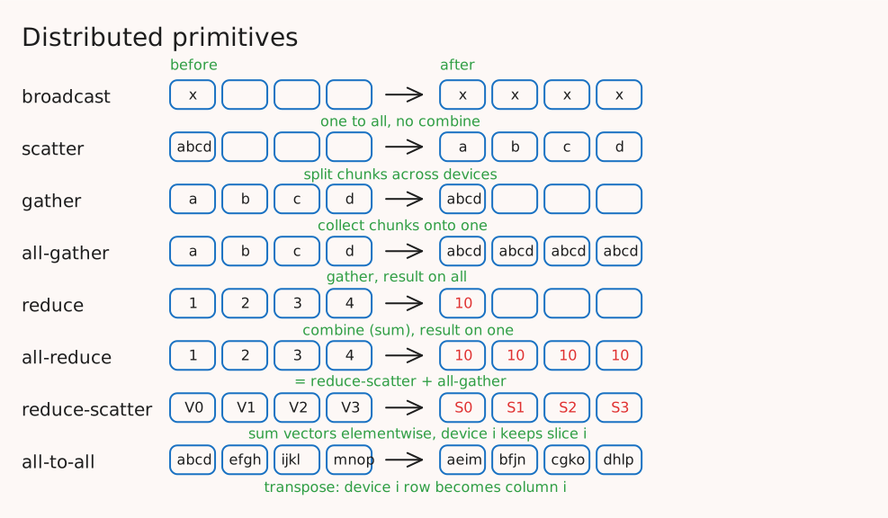
The four bold rows are the ones training uses constantly. All-reduce is the data-parallel gradient sync and the tensor-parallel sync. All-gather and reduce-scatter are what ZeRO and FSDP use to assemble and disassemble sharded state, and what sequence parallelism uses at its boundaries. All-to-all is the expert-parallel dispatch in mixture-of-experts models.
The ring algorithm, and where \((p-1)/p\) comes from
The volume column deserves a derivation, because the same factor shows up in every communication estimate for the rest of the post and it is not obvious where it comes from. The picture first, since the whole derivation is a walk through it:
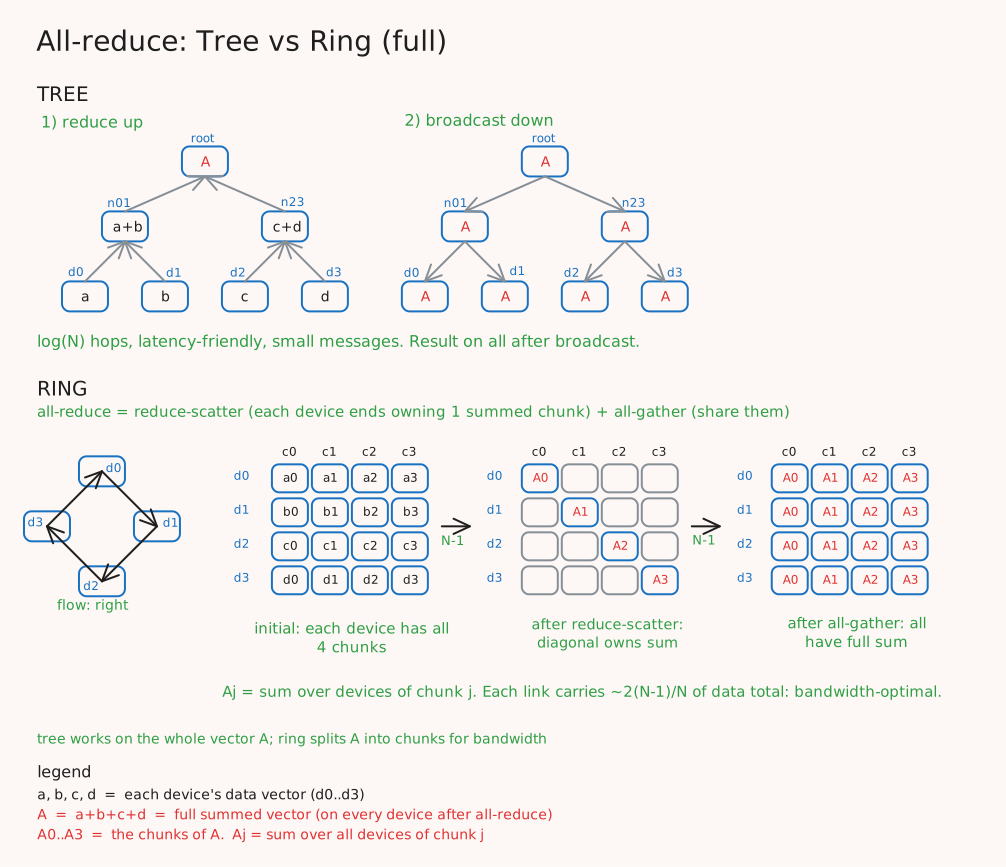
The setup. There are \(p\) devices (\(p = 4\) in the figure) and each holds its own vector of \(S\) bytes: \(d_0\) holds \(a\), \(d_1\) holds \(b\), and so on. In training, “its own vector” is that rank’s local gradient. Every vector is cut into \(p\) equal chunks of \(S/p\) bytes each, so \(a = (a_0, a_1, a_2, a_3)\), and in the ring’s left grid a row is a device and a column is a chunk index. The all-reduce has to produce the elementwise sum \(A = a + b + c + d\) on every device. Since the sum is elementwise, it can be done chunk by chunk: \(A_j = a_j + b_j + c_j + d_j\), and the right grid, every device holding \(A_0\) to \(A_3\), is the finished state.
The devices form a logical ring, \(d_0 \to d_1 \to d_2 \to d_3 \to d_0\), and each device only ever sends to its right neighbor and receives from its left. The algorithm has two phases.
Phase 1, reduce-scatter: \(p - 1\) steps. Give each device one chunk index to end up owning: device \(j\) will own chunk \(j\), which is the diagonal in the middle grid. Follow one chunk’s journey. \(A_1\) will end on \(d_1\), and its trip starts on the device after it: \(d_2\) sends its \(c_1\) to \(d_3\), which adds its own \(d_1\) and sends \(c_1 + d_1\) on to \(d_0\), which adds \(a_1\) and sends \(a_1 + c_1 + d_1\) to \(d_1\), which adds \(b_1\) and now holds \(A_1\). Three hops, three additions, one finished chunk. Every other chunk makes the same trip one device over: \(A_0\)’s trip starts at \(d_1\) and ends at \(d_0\), \(A_2\)’s starts at \(d_3\) and ends at \(d_2\), \(A_3\)’s starts at \(d_0\) and ends at \(d_3\). Because the four trips are staggered, at every step each device sends exactly one chunk and receives exactly one, so all four links are busy at once; that is the trick that makes the ring efficient. After \(p - 1 = 3\) steps the middle grid holds: device \(j\) has the complete \(A_j\), and the other chunks on each device are stale partial sums that are no longer needed.
Count the bytes for one device in this phase: \(p - 1\) steps, and in each step it sends one chunk of \(S/p\) bytes to its right neighbor and receives one from its left. Counting the sent side (the received side is identical):
\[(p-1)\,\frac{S}{p} = S\,\frac{p-1}{p}\]That is the reduce-scatter row of the table.
Phase 2, all-gather: \(p - 1\) more steps. Now the finished chunks circulate. In the first step \(d_1\) sends \(A_1\) to \(d_2\), \(d_2\) sends \(A_2\) to \(d_3\), and so on around the ring; in each later step every device forwards the chunk it just received. After \(p - 1\) steps each chunk has visited every device, and the right grid holds \(A_0\) to \(A_3\) everywhere. The byte count is the same as phase 1: \(p - 1\) chunks of \(S/p\) sent per device, \(S(p-1)/p\), the all-gather row.
Total. Two phases of \(p - 1\) steps, each step moving one \(S/p\)-byte chunk per device:
\[2\,(p-1)\,\frac{S}{p} = 2S\,\frac{p-1}{p}\]sent by each device, and the same amount received. The \((p-1)/p\) now has a plain reading: the answer has \(p\) chunks, and in each phase a device already holds one of them (the chunk it is reducing, or the finished chunk it owns), so it only has to move the other \(p - 1\). For \(p = 4\) that is \(3/4\) of \(S\) per phase and \(1.5\,S\) in total; for \(p = 8\), \(7/8\) and \(1.75\,S\); as \(p\) grows it approaches \(2S\). So a ring all-reduce costs each device about \(2S\) of traffic no matter how many devices take part, which is what lets it scale.
What “bandwidth-optimal” means. Patarasuk and Yuan prove that any all-reduce algorithm, however clever, must have at least one device that sends or receives \(2S(p-1)/p\) bytes (their Lemma 4, stated in data items). The ring hits that bound exactly, on every device at once. So if the time of a collective is set by how many bytes have to pass through the busiest link, nothing can beat the ring; it is optimal in the bandwidth term. That statement is only about bytes. It says nothing about how many sequential steps the algorithm takes, and that is exactly where the ring is weak, as the cost model below shows.
The tree, for contrast. The top half of the figure reduces the same four vectors up a binary tree: \(d_0\) and \(d_1\) send \(a\) and \(b\) (all four chunks at once) to an intermediate node that forms \(a + b\), likewise \(c + d\), then the root forms \(A_0\) to \(A_3\) and broadcasts it back down. It finishes in \(2\log_2 p\) hops, 4 for four devices against the ring’s \(2(p-1) = 6\), and 6 against 14 for eight. But every hop moves a whole \(S\)-byte vector, and the node under the root handles several vectors’ worth, so its busiest link carries more than the ring’s \(2S(p-1)/p\). Fewer, larger hops: latency-friendly and bandwidth-heavy, the mirror image of the ring.
The identity the ring makes visible, all-reduce \(=\) reduce-scatter \(+\) all-gather, is more than an implementation detail. It is the hinge the entire ZeRO family turns on: if an all-reduce is already two phases with a moment in the middle where each device holds one fully reduced chunk (the diagonal), then a device can do useful work on its chunk between the phases, and that is exactly where the sharded optimizer step goes. We’ll see it in the data parallelism section.
The cost model: latency, bandwidth, throughput
Three words that are easy to mix up, so a mental model first. Think of a link between two GPUs as a water pipe.
| Term | Symbol | What it is | Pipe picture |
|---|---|---|---|
| Latency | \(\alpha\) | the fixed time between sending a message and its first byte arriving, whatever its size: handshake, kernel launch, switch hops | how long after you open the tap before any water comes out the far end |
| Bandwidth | \(B\) | the rate at which the link carries bytes once they are flowing, a property of the hardware: 450 GB/s per direction for NVLink, 50 GB/s for 400 Gb/s InfiniBand | the pipe’s diameter |
| Throughput | what you actually achieved: bytes delivered divided by the time it took, including the waiting | how much water you collected per second, from tap-open to tap-close |
Bandwidth is the ceiling; throughput is what a particular transfer got. For one message of \(n\) bytes, the time is
\[T(n) = \alpha + \frac{n}{B}\]and the throughput is \(n / T(n)\). A tiny message spends almost all of its time in \(\alpha\) and its throughput is a small fraction of \(B\); a huge message spends almost all of its time in \(n/B\) and its throughput approaches \(B\). The two terms are equal at \(n = \alpha B\), the message size at which half the time is waiting: for every microsecond of latency on a 450 GB/s link, that crossover is \(450\) KB. Messages far below \(\alpha B\) are latency-bound (the link is mostly idle), messages far above it are bandwidth-bound (the link is mostly full). Note that \(n\) here is one message; it is not the \(S\) of the previous subsection, which was the whole vector being reduced.
Now apply this to the ring. It runs \(2(p-1)\) sequential steps, and each step is one message of \(S/p\) bytes, so:
\[T_{\text{ring}} = 2(p-1)\left(\alpha + \frac{S}{pB}\right) = \underbrace{2(p-1)\,\alpha}_{\text{latency term}} + \underbrace{2\,\frac{p-1}{p}\,\frac{S}{B}}_{\text{bandwidth term}}\]The bandwidth term is the optimal one from above. The latency term is paid once per step, and there are \(2(p-1)\) steps, so it grows linearly with the number of devices; Patarasuk and Yuan say exactly this, that the ring is optimal in the bandwidth term but not the latency term. A tree pays \(\alpha\) only \(2\log_2 p\) times. Which term matters depends on \(S\), and the dividing line comes from setting the two terms equal: \(2(p-1)\alpha = 2\frac{p-1}{p}\frac{S}{B}\) gives \(S = p\,\alpha B\), the single-message crossover \(\alpha B\) scaled by \(p\) because each step’s message is only \(S/p\):
| Regime | When | What \(T_{\text{ring}}\) looks like | What helps |
|---|---|---|---|
| Latency-bound | \(S\) is small, well under \(p\,\alpha B\) | \(\approx 2(p-1)\alpha\): independent of \(S\), grows with \(p\) | send fewer messages: bucket many small tensors into one collective; use tree-shaped algorithms with fewer steps |
| Bandwidth-bound | \(S\) is large, well over \(p\,\alpha B\) | \(\approx 2S/B\): independent of \(p\), proportional to \(S\) | move fewer bytes (smaller dtype, sharding), use a faster link, or overlap the transfer with compute |
Read the two “independent of” notes slowly, because they are the point. In the latency-bound regime, making the vector smaller does nothing and adding devices makes it worse. In the bandwidth-bound regime, adding devices costs nothing extra (that is the ring’s optimality at work) and the only lever is the number of bytes over the link’s speed.
Why gradient bucketing matters. A transformer’s gradient is not one vector; it is hundreds of separate tensors, one per weight matrix, bias, and norm, and many of them are tiny: a norm’s weight vector on the 70B model is \(8192\) elements, 16 KB in bf16, far below any plausible \(\alpha B\). All-reducing each tensor on its own would pay the full latency term, \(2(p-1)\alpha\), hundreds of times per step, and most of those calls would be pure waiting. Bucketing concatenates the tensors into a few large buffers and runs one collective per buffer. PyTorch’s DDP uses 25 MiB buckets by default; at that size each collective is deep in the bandwidth-bound regime, so the total time is close to (total gradient bytes) \(/ B\) no matter how many tensors the model has. The next section shows how DDP does this on the fly during the backward pass.
A worked number
To set the scale, all-reduce the 70B model’s bf16 gradient. Every rank holds its own copy, \(S = 70 \times 10^9 \times 2 = 140\) GB.
Eight GPUs in one node, over NVLink. Each chunk is \(S/p = 140/8 = 17.5\) GB. The reduce-scatter is 7 steps of one chunk each, \(7 \times 17.5 = 122.5\) GB sent per rank; the all-gather is another 7 steps and another 122.5 GB; total \(245\) GB sent and 245 GB received per rank, which is the formula’s \(2 \times 7/8 \times 140\). Every rank sends over its own link at the same time, so the collective takes as long as one rank’s traffic, not the sum over ranks: \(245 / 450 \approx 0.54\) s at 450 GB/s per direction. The latency term is invisible here; 14 steps of \(\alpha\) are microseconds against half a second.
Sixty-four GPUs across eight nodes, over 400 Gb/s InfiniBand. First the units: InfiniBand is quoted in gigabits per second, and 400 Gb/s is \(400 / 8 = 50\) GB/s per direction, which is the figure the bandwidth ladder uses and the one to divide by. Each chunk is \(140/64 = 2.19\) GB; 63 steps per phase, \(63 \times 2.19 = 138\) GB per phase, \(276\) GB in total per rank, the formula’s \(2 \times 63/64 \times 140\). The per-rank bytes barely moved (the ring is bandwidth-optimal, so adding ranks did not add traffic), but the link is nine times slower than NVLink’s 450 GB/s: \(276 / 50 \approx 5.5\) s.
Half a second to five seconds, per step, for one collective. Those are the numbers that have to be hidden behind compute for data parallelism to work at all, and hiding them is the next section’s main subject.
Overlap is the whole game
A collective that runs while the GPU is otherwise idle is fully exposed: its time adds directly to the step. A collective that runs while the GPU computes something else is free, up to the bandwidth of the link. Every well-designed training system is built around finding compute to hide each collective behind. Stated here only as a principle; each of the following is worked out in its own section:
- DDP launches the all-reduce of one bucket of gradients while the backward pass is still computing the gradients of earlier layers.
- FSDP all-gathers the parameters of layer \(i+1\) while layer \(i\) computes.
- Pipeline parallelism sends activations to the next stage asynchronously while the current stage keeps working on the next microbatch.
- Tensor parallelism is the hardest to hide, which is why it is placed on the fastest link rather than overlapped away.
If a system is not overlapping, the communication is visible directly as a gap in a profiler timeline, with the GPU’s compute streams empty while the network interface is busy. Most of what follows is arranging for those gaps not to exist.
References
- Bandwidth Optimal All-reduce Algorithms for Clusters of Workstations - Patarasuk and Yuan, JPDC 2009
- Bringing HPC Techniques to Deep Learning - Gibiansky (the ring all-reduce walkthrough)
- NCCL collective operations (the semantics of each primitive)
- PyTorch Distributed: Experiences on Accelerating Data Parallel Training - Li et al. (bucketing)
Data Parallelism
Data parallelism is the oldest and simplest way to use more GPUs: give each one a copy of the model and a different slice of the batch. It is also where the 16-bytes-per-parameter problem bites hardest, and the ZeRO family is the response. This section builds up from the plain version.
Vocabulary: batch, microbatch, and the letters
From here on the word “batch” is doing several jobs, and the parallelism sections that follow lean on the distinctions, so here they are in one place:
| Term | Symbol | Meaning |
|---|---|---|
| Global batch | the data consumed per optimizer step, across all ranks; the number the optimizer cares about. Llama 3 uses 16M tokens (Table 4) | |
| Data-parallel degree | \(D\) | how many ranks process different data in parallel; each holds a full replica (DDP) or a shard of one (ZeRO, FSDP) |
| Batch per rank | global \(/ D\) | the share of the global batch one data-parallel rank is responsible for each step; Llama 3’s “batch per DP rank” of 32 is 32 sequences of 8,192 tokens |
| Hidden dimension | \(h\) | the width of one token’s activation row: a token is a row of \(h\) values, and every matmul in the layer multiplies rows of this width (\(h = 8192\) for Llama 3 70B). Not a batch quantity, but it sits next to the two below in every formula |
| Microbatch | a tensor of shape \((b, s, h)\) | what one rank pushes through one forward and backward pass at a time: \(b\) sequences, each of \(s\) tokens, each token a row of \(h\) values, so \(b \times s\) token rows go through the matmuls together. These are the \(b\), \(s\), \(h\) of the activation formula, and the microbatch is what activation memory limits |
| Accumulation steps | \(k\) | microbatches per rank per optimizer step, so batch per rank \(= b \times k\); under pipeline parallelism these same microbatches are the pipeline’s \(m\) |
| Ranks in a collective | \(p\) | the number of participants in whatever collective is being costed (the primitives section); for a data-parallel gradient sync, \(p = D\). The pipeline section reuses \(p\) for the number of stages, and says so |
The one relation to keep in mind: global batch \(= D \times b \times k\) sequences, or \(D \times b \times k \times s\) tokens. The optimizer sees the left side; activation memory sees only the one \((b, s, h)\) microbatch in flight; communication is paid once per step, whatever \(k\) is.
Distributed data parallel
In plain distributed data parallel (DDP), every rank holds a full replica of the model, the optimizer state included. Each step, every rank runs the forward and backward pass on its own microbatch, producing a local gradient. The gradients are then averaged across ranks with an all-reduce, so that every rank holds the same gradient, the gradient of the loss over the whole global batch. Every rank then applies the same optimizer update to its identical copy of the weights, and the replicas stay in lockstep without ever exchanging weights (Li et al., Section 3).
The mechanics that make this fast are in PyTorch’s implementation, and they are a direct application of the cost model above:
- Hooks, not a barrier. DDP registers an autograd hook on every parameter. When that parameter’s gradient is computed during the backward pass, the hook fires and marks it ready. There is no “wait for the whole backward pass, then all-reduce everything.”
- Buckets. Parameters are grouped into buckets of a fixed size, 25 MiB by default (
bucket_cap_mb, DDP docs), in roughly the reverse of the model’s parameter order, because the backward pass produces gradients for the last layers first. When every gradient in a bucket is ready, DDP launches one asynchronous all-reduce for the whole bucket. - Overlap. Because the all-reduce of a ready bucket runs while autograd is still computing gradients for earlier layers, most of the communication hides behind the backward pass. Only the last bucket’s all-reduce is necessarily exposed. The paper reports that this overlap, plus the bucketing, is what turns a naive implementation into a scalable one (Section 3.2.3).
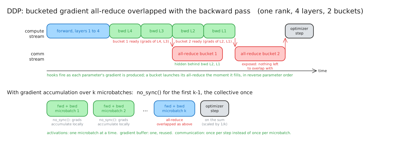
The cost of DDP per step is one all-reduce over the entire gradient, \(2S(p-1)/p\) per rank with \(S\) the gradient bytes, most of it hidden. The memory cost is the problem: every rank holds the full 16 bytes per parameter, and adding ranks does nothing about it. A 70B model needs 1.12 TB per GPU under plain DDP, whether there are 8 GPUs or 8,000.
Gradient accumulation
Before fixing the memory problem, one knob that is independent of it. The batch size a run wants for optimization reasons (Llama 3 uses 16M tokens per batch, Table 4) is far larger than what fits through a GPU in one forward pass, since activations scale with the batch. Gradient accumulation decouples the two.
The gradient of a mean loss over a batch is the mean of the gradients over its parts. If the global batch is split into \(k\) equal microbatches, then:
\[\nabla L_{\text{batch}} = \frac{1}{k}\sum_{j=1}^{k} \nabla L_{\text{microbatch}\,j}\]So a rank can run the forward and backward pass \(k\) times, on \(k\) different microbatches, adding each backward pass’s gradient into the same gradient buffer instead of zeroing it, and only then take one optimizer step on the accumulated sum (scaled by \(1/k\), or equivalently with the per-microbatch losses pre-scaled). Three things follow:
- Memory. Only one microbatch’s activations are alive at a time, so the activation footprint is that of a microbatch, not the batch. The gradient buffer is the same size regardless. This is the entire point.
- Effective batch. The optimizer sees a batch of \(\text{DP} \times \text{microbatch size} \times k\). Megatron-LM’s
--global-batch-sizeand--micro-batch-sizeflags are exactly this pair, with \(k\) derived from them and the data-parallel degree (megatron/training/arguments.py). - Communication. The gradient all-reduce should happen once per optimizer step, not once per microbatch. Under DDP, every backward pass would trigger the bucketed all-reduces by default, so DDP provides a
no_sync()context manager that disables them; run the first \(k-1\) microbatches inside it and the last one outside, and the collective runs once, amortized over \(k\) microbatches (Li et al., Section 3.2.4). FSDP has the same context manager with one twist: insideno_sync()the accumulated gradients are kept unsharded on every rank, so the memory saving of sharding is temporarily given up in exchange for the communication saving (FSDP docs).
There is one more identity worth stating now and returning to later: under pipeline parallelism, the microbatches that fill the pipeline are the gradient-accumulation microbatches. The pipeline’s \(m\) and the accumulation’s \(k\) are the same number, which is why choosing it is a throughput decision (the bubble) and a memory decision (activations in flight) at once.
ZeRO: removing the redundancy
Look at what the \(p\) replicas in DDP are holding. Every rank has the same optimizer state, the same master weights, the same gradients after the all-reduce, and the same weights. Everything but the activations is replicated \(p\) times. ZeRO (Rajbhandari et al.) partitions that state so each rank holds only \(1/p\) of it, in three stages of increasing aggressiveness. Let \(D\) be the data-parallel degree and \(\Psi\) the parameter count:
| Stage | What is partitioned | Bytes per parameter per rank | Communication per step, relative to DDP |
|---|---|---|---|
| Baseline DDP | nothing | \(16\) | \(1\times\) (one all-reduce, \(2\Psi\) elements) |
| ZeRO-1 (\(P_{os}\)) | optimizer state: master weights, \(m\), \(v\) | \(4 + \dfrac{12}{D}\) | \(1\times\) |
| ZeRO-2 (\(P_{os+g}\)) | plus gradients | \(2 + \dfrac{14}{D}\) | \(1\times\) |
| ZeRO-3 (\(P_{os+g+p}\)) | plus parameters | \(\dfrac{16}{D}\) | \(1.5\times\) (\(3\Psi\) elements) |
The memory column is the paper’s Figure 1 and Section 5; the communication column is its Section 7. What the mechanics look like at each stage:
ZeRO-1 is the ring identity from the previous section put to work. Instead of an all-reduce, do a reduce-scatter of the gradients: afterwards rank \(i\) holds the fully summed gradient for its \(1/D\) slice of the parameters and nothing else. Rank \(i\) owns the master weights and Adam moments for exactly that slice, so it runs the optimizer step on its slice alone. Then all-gather the updated 16-bit weights so every rank has the full model again for the next forward pass. Reduce-scatter plus all-gather moves \(\Psi + \Psi = 2\Psi\) elements, the same as the all-reduce it replaced, and the optimizer state, 12 of the 16 bytes, is now divided by \(D\). Nearly a 4x memory reduction for free, which is why this stage is close to universal; Megatron-LM’s --use-distributed-optimizer is the same idea.
ZeRO-2 notices that after the reduce-scatter a rank only needs the gradient of its own slice, so gradients can be reduced bucket by bucket during the backward pass and discarded once they are reduced to their owner. The gradient’s 2 bytes drop to \(2/D\). The communication volume is unchanged.
ZeRO-3 partitions the parameters themselves, so no rank ever holds the full model. That means a rank has to all-gather each layer’s parameters right before it needs them in the forward pass, run the layer, and free the gathered copy; then all-gather them again in the backward pass, since the weights were freed after the forward. Two all-gathers of \(\Psi\) plus the reduce-scatter of \(\Psi\) is \(3\Psi\) elements, and \(3\Psi / 2\Psi\) is the \(1.5\times\). In exchange, everything, all 16 bytes, is divided by \(D\).
Run the 70B model on 64 GPUs through the table (16-bit gradients, \(\Psi = 70 \times 10^9\)):
| Stage | Static memory per GPU |
|---|---|
| DDP | \(16 \times 70 = 1{,}120\) GB |
| ZeRO-1 | \((4 + 12/64) \times 70 = 293\) GB |
| ZeRO-2 | \((2 + 14/64) \times 70 = 155\) GB |
| ZeRO-3 | \((16/64) \times 70 = 17.5\) GB |
Only ZeRO-3 fits in 80 GB, and it fits with room for activations. Notice that ZeRO-1 and ZeRO-2 are capped by the 4 and 2 bytes that stay replicated, so no number of GPUs makes them fit a 70B model on an 80 GB card; only ZeRO-3 scales the whole footprint with \(D\). And notice the flip side: at \(D = 8\), ZeRO-3 gives \(140\) GB per GPU, which still does not fit, so a single node cannot train a 70B model with data parallelism alone. That is the seam where model parallelism, the next two sections, takes over.
FSDP: ZeRO-3 as the PyTorch engine builds it
PyTorch’s FullyShardedDataParallel is the same idea as ZeRO’s third stage, and its paper describes the engineering that makes the \(1.5\times\) communication survivable (Zhao et al.):
- Units and flat parameters. The model is divided into units, typically one transformer layer each. All the parameters of a unit are flattened into one contiguous 1-D
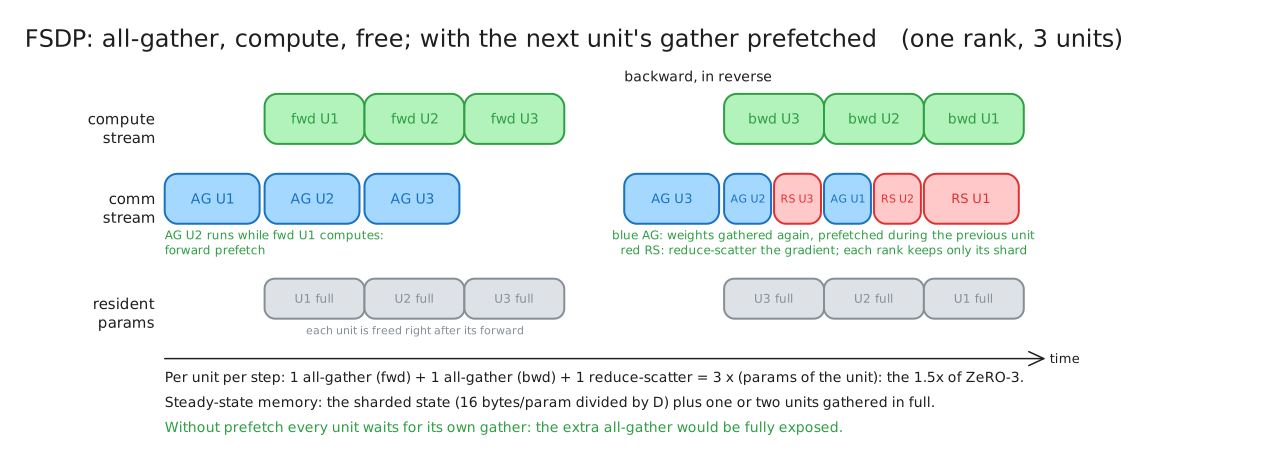
FlatParameter, which is chunked evenly across ranks. One unit is one all-gather, which keeps the collective count low and each collective large, per the cost model. - The lifecycle. For each unit, in order: all-gather its flat parameter, run the forward, free the peer shards. In the backward pass: all-gather again, run the backward, reduce-scatter the gradient so each rank keeps the shard it owns, free. After the backward, each rank holds sharded parameters, sharded gradients, and sharded optimizer state, and runs the optimizer step on its shard.
- Prefetching. The all-gather for unit \(i+1\) is issued before unit \(i\)’s compute finishes (forward prefetch), and in the backward pass the next unit’s all-gather is issued ahead of the current unit’s reduce-scatter (backward prefetch, Sections 3.3.2 and 3.3.3). This is the overlap that hides the extra all-gather. Without it, every layer would wait on its own parameters arriving over the network, and the extra \(\Psi\) of communication would be fully exposed. The sentence to remember: FSDP is viable because the gather for the next layer overlaps the compute of the current one.
Two practical variants are worth knowing.
Keep the weights after the forward pass. Llama 3 uses FSDP as its outermost parallelism and does not reshard the parameters after the forward pass, keeping the gathered weights around so the backward pass needs no second all-gather (Section 3.3.2): communication back down to \(2\Psi\), memory back up by the gathered weights, a trade that makes sense when the other parallelism dimensions have already made each rank’s share of the weights small.
Hybrid sharding. Full sharding across all \(W\) ranks puts the \(3\Psi\) of all-gather and reduce-scatter traffic on whatever link connects the farthest ranks, which across nodes is the slow one. Hybrid sharding (Zhao et al., Section 3.2) picks a sharding factor \(F\) smaller than \(W\), say \(F = 8\) for one node, shards each parameter only within groups of \(F\) ranks, and replicates across the \(W/F\) groups. Two things change:
- Memory. Each rank now holds \(1/F\) of the state rather than \(1/W\): the 16 bytes per parameter are divided by 8, not by 64. For the 70B model that is 140 GB per GPU, which does not fit, so on its own hybrid sharding suits models that are only somewhat too large to replicate; for larger models it is combined with tensor and pipeline parallelism, which shrink each group’s share first.
- Communication. The all-gathers and the reduce-scatter, the traffic that made ZeRO-3 cost \(1.5\times\) DDP, now run inside the node over NVLink. What crosses the network is only the last step of the gradient reduction: after each group has reduce-scattered, every rank holds a \(\Psi/F\) gradient shard that must still be averaged with the same shard on the other \(W/F\) replicas, one all-reduce of \(\Psi/F\) elements. The paper states the equivalence directly: the single reduce-scatter over all ranks becomes a reduce-scatter within each sharded group followed by an all-reduce within each replicated group.
Put numbers on it for the 70B model on 64 GPUs. Fully sharded across all 64, each rank moves about \(3 \times 140 \times 63/64 = 413\) GB per step, much of it across InfiniBand at 50 GB/s, on the order of 8 s if exposed. Hybrid with \(F = 8\): the in-node part is \(3 \times 140 \times 7/8 = 368\) GB per rank at 450 GB/s, about 0.8 s, and the cross-node part is an all-reduce of a \(140/8 = 17.5\) GB shard across 8 replicas, \(2 \times 7/8 \times 17.5 = 31\) GB per rank at 50 GB/s, about 0.6 s. The slow link carries a twelfth of the bytes it did, at the price of holding eight times the state per GPU. That is the trade hybrid sharding offers, and it is the same rule as everywhere else in this post: put the heavy traffic on the fast link.
Offloading
If the state still does not fit, it can leave the GPU. ZeRO-Offload keeps the 16-bit parameters and the forward and backward computation on the GPU but moves the fp32 master weights, the Adam moments, and the 16-bit gradients to host memory, where a CPU implementation of Adam runs the update (Ren et al.). ZeRO-Infinity extends the same idea on top of ZeRO-3, spilling parameters and optimizer state across GPU, CPU, and NVMe (Rajbhandari et al. 2021).
The price is on the bandwidth ladder: PCIe Gen5 moves 64 GB/s per direction, seven times less than NVLink and fifty times less than HBM. Offloading is the right call when the run is capacity-bound and has wall-clock to spare (fine-tuning a large model on few GPUs); it is the wrong call when the run is already communication-bound, because it adds the slowest link in the machine to the critical path.
References
- PyTorch Distributed: Experiences on Accelerating Data Parallel Training - Li et al., DistributedDataParallel docs
- ZeRO: Memory Optimizations Toward Training Trillion Parameter Models - Rajbhandari et al.
- PyTorch FSDP: Experiences on Scaling Fully Sharded Data Parallel - Zhao et al., FSDP docs
- ZeRO-Offload - Ren et al., ZeRO-Infinity - Rajbhandari et al.
- The Llama 3 Herd of Models
- Megatron-LM arguments
Tensor Parallelism
Data parallelism splits the batch. Tensor parallelism (TP) splits the model, one weight matrix at a time, so that each rank holds a slice of every matrix and the ranks cooperate on every layer. The scheme every framework uses is Megatron-LM’s (Shoeybi et al.), and its cleverness is entirely in which way each matrix is cut.
The MLP: column, then row
The transformer MLP is two matmuls with a nonlinearity between them:
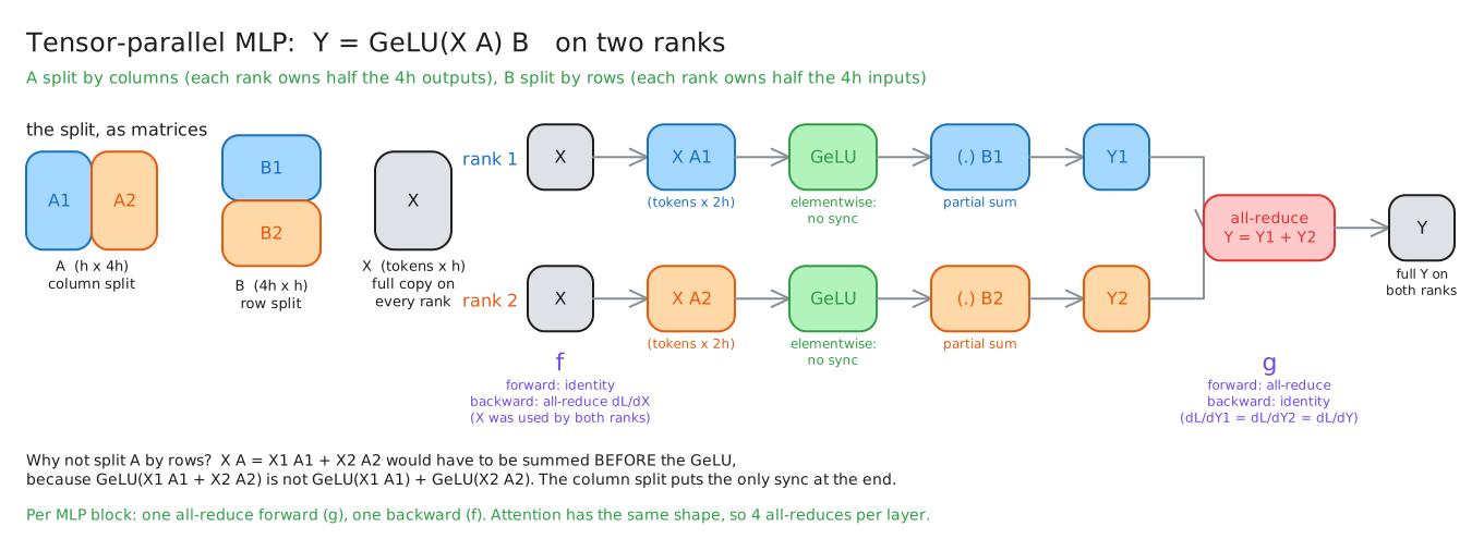
\[Y = \mathrm{GeLU}(X A)\, B\]with \(X\) of shape \((\text{tokens} \times h)\), \(A\) of shape \((h \times 4h)\), and \(B\) of shape \((4h \times h)\). Suppose two ranks. There are two ways to cut \(A\) in half:
Cut \(A\) along its rows (the \(h\) dimension, the one the matmul contracts over). Then \(X\) has to be cut the same way, and \(XA = X_1 A_1 + X_2 A_2\): each rank produces a partial sum, and the two have to be added before the GeLU, because
\[\mathrm{GeLU}(X_1 A_1 + X_2 A_2) \neq \mathrm{GeLU}(X_1 A_1) + \mathrm{GeLU}(X_2 A_2)\]GeLU is nonlinear, so it cannot be pushed through a sum. A row split forces a synchronization in the middle of the block.
Cut \(A\) along its columns (the \(4h\) dimension). Then \(XA = [\,X A_1 \;\; X A_2\,]\): each rank takes the full \(X\) and produces its own half of the columns, and since GeLU is elementwise it applies to each half independently: \([\,\mathrm{GeLU}(X A_1) \;\; \mathrm{GeLU}(X A_2)\,]\). No communication. This is why the first matrix is split column-wise (Shoeybi et al., Section 3, Eq. 1 to 3), and it is the detail the whole design rests on.
Now the second matmul. The output of the first is column-split, which means each rank holds a slice of the \(4h\) dimension, and that is exactly the dimension \(B\) contracts over. So cut \(B\) along its rows to match: rank \(i\) computes \(Y_i = \mathrm{GeLU}(X A_i)\, B_i\) from purely local data, and
\[Y = Y_1 + Y_2\]One all-reduce sums the partials and every rank holds \(Y\). Column-then-row is the pairing that puts the single unavoidable sync at the end of the block rather than in the middle of it.
The \(f\) and \(g\) operators
Megatron writes the communication as two operators placed at the block’s boundaries (Figure 3):
| Operator | Forward pass | Backward pass | Where |
|---|---|---|---|
| \(f\) | identity (every rank already has the full \(X\)) | all-reduce | entering the block |
| \(g\) | all-reduce (sum the \(Y_i\)) | identity | leaving the block |
They are called conjugates, and the reason each has the backward it has is worth seeing rather than memorizing. \(g\)’s backward is an identity because \(Y = Y_1 + Y_2\) means \(\partial L / \partial Y_i = \partial L / \partial Y\) for every \(i\); each rank already holds the incoming gradient and just uses it. \(f\)’s backward is an all-reduce because \(X\) was used by every rank, each computing its own \(X A_i\), and a value used in several places accumulates the gradient from each use. That is the fork rule from the LayerNorm post, applied across GPUs: \(\partial L / \partial X\) is the sum over ranks of each rank’s local contribution, and summing across ranks is an all-reduce.
So the MLP block costs one all-reduce in the forward pass and one in the backward pass.
Attention: split by heads
Multi-head attention has the same two-matmul shape, and heads make the split natural. The query, key, and value projections are cut column-wise, so that rank \(i\) ends up holding whole heads: with \(a\) heads and \(t\) ranks, \(a/t\) complete heads per rank, each with its full \(Q\), \(K\), and \(V\) for those heads. Everything inside attention, the scores, the softmax over keys, the weighted sum over values, happens within a head, so each rank runs attention for its own heads with no communication at all. The output projection \(W_O\) contracts over the concatenated-heads dimension, which is exactly the dimension that is now sharded, so it is cut row-wise, and one all-reduce sums the ranks’ partial outputs (Shoeybi et al., Figure 3b). Same \(f\) and \(g\), same one-all-reduce-per-direction.
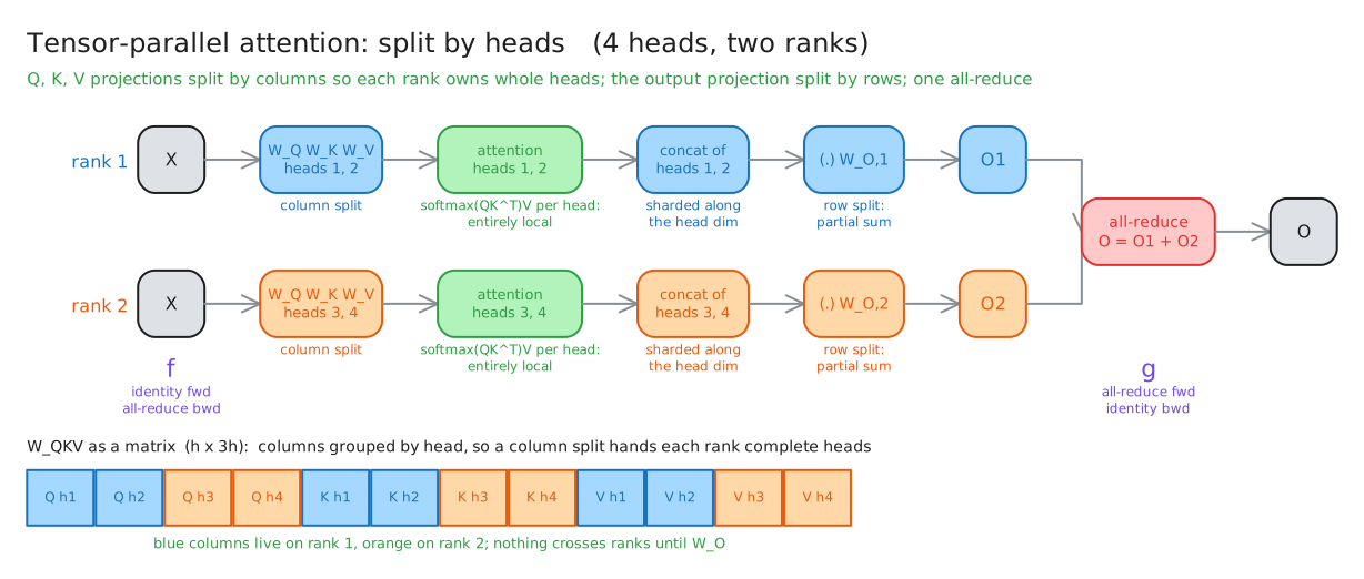
Putting the two blocks together, a tensor-parallel transformer layer costs two all-reduces in the forward pass and two in the backward pass, four communication operations per layer (Figure 4). The layer norms, dropouts, and residual additions that sit between the blocks are not split; every rank computes them redundantly on the full hidden state, which is cheaper than communicating and is the redundancy sequence parallelism will remove below.
What the four all-reduces cost
Each all-reduce is over the hidden state for one microbatch: a \(b \times s \times h\) tensor, \(S = 2\,b\,s\,h\) bytes in bf16. From the ring analysis, each rank sends and receives \(2S(t-1)/t\) per all-reduce, and there are four per layer, so per layer per rank per microbatch:
\[4 \times 2 \times 2\,b\,s\,h \times \frac{t-1}{t} \;=\; 16\,b\,s\,h\,\frac{t-1}{t} \text{ bytes}\]Take the 70B model (\(h = 8192\), 80 layers) with \(b \times s = 8192\) tokens per microbatch and \(t = 8\). One hidden-state tensor is \(2 \times 8192 \times 8192 = 134\) MB. Then:
| Quantity | Value |
|---|---|
| Per all-reduce, per rank | \(2 \times 134 \text{ MB} \times 7/8 = 235\) MB |
| Per layer (4 all-reduces) | \(0.94\) GB |
| Per microbatch, 80 layers | 75 GB sent and received per rank |
| Time on NVLink, 450 GB/s per direction | \(\approx 0.17\) s |
| Time on PCIe Gen5, 64 GB/s | \(\approx 1.2\) s |
| Time on 400 Gb/s InfiniBand, 50 GB/s | \(\approx 1.5\) s |
Compare that with the compute for the same microbatch: \(6 \times 70 \times 10^9 \times 8192 = 3.4 \times 10^{15}\) FLOPs spread over 8 GPUs at 989 TFLOPS each is about \(0.43\) s at 100% utilization and about \(1.1\) s at a realistic 40%.
Why tensor parallelism stays inside the node
The table above is the whole argument, but it is worth walking through slowly, because “TP stays in the node” is the single most consequential placement rule in this post and it should feel inevitable rather than remembered.
First, the traffic is on the critical path. The four all-reduces per layer are not background work. Each one sits between two matmuls that depend on it: the row-parallel matmul produces partial sums, the all-reduce adds them, and the next block cannot start until the sum exists, because its input is that sum. So every layer, twice per direction, the GPUs stop computing and wait for a collective to finish. Unlike the data-parallel gradient sync, which can hide behind the backward pass, there is very little compute to hide a tensor-parallel all-reduce behind. Its time adds almost directly to the step. (Megatron has a --tp-comm-overlap option that recovers part of it by splitting the matmul and overlapping pieces, but the dependency is structural.)
Second, there are a lot of them. Four per layer times 80 layers is 320 all-reduces per microbatch, in the forward and backward passes together, each on a hidden-state tensor of \(b \times s \times h\) elements. That is what produced the 75 GB per rank per microbatch above.
Third, put the bytes on each rung of the bandwidth ladder and compare with the compute of the same microbatch:
| Link | One-way bandwidth | Time for the 75 GB | Against about 1.1 s of compute |
|---|---|---|---|
| NVLink, inside the node | 450 GB/s | 0.17 s | a sizable tax, partly recoverable by overlap |
| PCIe Gen5 | 64 GB/s | 1.2 s | longer than the compute itself |
| InfiniBand, across nodes | 50 GB/s | 1.5 s | longer than the compute itself |
Inside the node the all-reduces cost a noticeable fraction of the step and are worth engineering around. Across nodes they would take longer than all of the arithmetic they are interleaved with; the GPUs would spend most of every layer waiting on the network, and adding more of them would make it worse. That is the sense in which tensor parallelism cannot leave the node: not that it is impossible, but that its 320 synchronizations per microbatch are only affordable on a link fast enough to make each one short.
Fourth, this is what the Megatron authors found, and said. Their communication analysis gives the per-layer tensor-parallel volume as \(8bsh(t-1)/t\) per device per microbatch, and they state that when \(t\) is larger than the number of GPUs in a single node, performing tensor parallelism across the slower inter-node links can be impractical (Narayanan et al., Section 3.2). They then measured it, sweeping tensor-parallel and pipeline-parallel sizes for a fixed 64-GPU budget, and throughput per GPU peaks when the tensor-parallel size equals the number of GPUs in a node, 8 on their DGX A100 nodes, and falls off beyond it (Section 5.4.1, Figure 13).
So the rule. Tensor parallelism is set to at most the number of GPUs that share NVLink, 8 on a DGX-class node, and never more. If the model still does not fit at TP 8, the answer is a different dimension, pipeline parallelism, whose communication is one activation per stage boundary rather than four all-reduces per layer, and which therefore tolerates the slow link. Llama 3’s configuration table has TP at exactly 8 in every row for this reason, and the composition section builds the rest of the placement on top of it.
The next section picks up the redundancy this leaves behind, the norm and dropout activations replicated on every rank, and the two other dimensions that split along the sequence and across experts.
References
- Megatron-LM: Training Multi-Billion Parameter Language Models Using Model Parallelism - Shoeybi et al.
- Efficient Large-Scale Language Model Training on GPU Clusters Using Megatron-LM - Narayanan et al.
- Megatron-LM README
- LayerNorm and RMSNorm - the fork rule
Sequence, Context, and Expert Parallelism
The four dimensions so far, data, tensor, and (next section) pipeline parallelism, split the batch, the matrices, and the layer stack. Three more dimensions split along axes those leave untouched, and each exists because one of the earlier accountings left a term behind:
| Dimension | What it splits | The term it attacks | Communication it adds |
|---|---|---|---|
| Sequence parallelism (SP) | the norm and dropout activations between tensor-parallel blocks, along the sequence, within a TP group | the \(10\,sbh\) that TP replicates on every rank | none beyond TP’s (an all-reduce becomes a reduce-scatter plus an all-gather) |
| Context parallelism (CP) | the whole sequence, for every layer, across a CP group | the \(b \times s\) activation scaling when \(s\) itself is too large | \(K\) and \(V\) exchanged between ranks in attention |
| Expert parallelism (EP) | the experts of a mixture-of-experts layer across an EP group | the parameter count of a model whose weights are mostly experts each token never touches | two all-to-alls per MoE layer, dispatch and combine |
Sequence parallelism: the 10 that tensor parallelism leaves behind
Look again at the per-layer activation formula with \(t\)-way tensor parallelism from the recomputation section, \(sbh(10 + 24/t + 5as/(ht))\). The \(24/t\) and the attention term shrink with \(t\); the 10 does not. Those 10 bytes per element are the activations in the parts of the layer tensor parallelism does not touch, the layer norm inputs, the dropout masks, the residual stream, which every rank computes and stores in full. At \(t = 8\) they are more than a third of the remaining activation memory.
Korthikanti et al. observe that those operations are pointwise along the sequence: a layer norm of token 5 does not depend on token 6. So the non-tensor-parallel regions can be split along the sequence dimension instead, each rank holding \(s/t\) tokens of the full hidden state. The catch is at the boundaries, where the tensor-parallel matmuls need the whole sequence:
| Boundary | Without sequence parallelism | With sequence parallelism |
|---|---|---|
| Entering a TP block (\(f\)) | identity forward, all-reduce backward | all-gather forward (assemble the full sequence), reduce-scatter backward |
| Leaving a TP block (\(g\)) | all-reduce forward, identity backward | reduce-scatter forward (sum the partials and hand each rank its sequence slice), all-gather backward |
The paper names the new pair \(g\) and \(\bar g\). The point is that an all-reduce is a reduce-scatter plus an all-gather, so replacing one all-reduce with one of each moves exactly the same number of bytes: sequence parallelism costs no extra communication, and the paper’s measurement is that it is slightly faster (the \(-3\)% in the recomputation section’s table), since the pointwise ops now run on \(1/t\) of the data. What it buys is the 10 becoming \(10/t\), so the per-layer formula becomes \(\frac{sbh}{t}(34 + 5as/h)\): every term divided by \(t\). In Megatron-LM it is the --sequence-parallel flag, and it only makes sense together with tensor parallelism, which is why the arguments file disables it when \(t = 1\).
The phrase to hold onto: same communication volume, strictly less activation memory.
Context parallelism: when the sequence is the problem
Sequence parallelism splits only the cheap regions between tensor-parallel blocks. Context parallelism (CP) splits the input sequence itself, so that with \(\text{CP} = c\) each rank holds a contiguous chunk of \(s/c\) tokens through every layer. Almost every operation in a transformer layer is per-token, the norms, the MLP, the QKV and output projections, so they all run unchanged on a chunk and never need to know the other chunks exist (Megatron Core context parallelism). Activation memory per rank, including the quadratic attention term, drops by \(c\). That is the memory story, and it is why CP is the dimension that unlocks 128K-token training: Llama 3 uses \(\text{CP} = 16\) for its long-context stage and 1 elsewhere (Table 4).
The one operation that is not per-token is attention. Each query has to see the keys and values of the whole sequence, and under CP the \(K\) and \(V\) for the other chunks live on other ranks. There are three ways to bring them together, and all three are in production:
| Method | Mechanism | Communication | Trade |
|---|---|---|---|
Ring (Ring Attention; Megatron p2p) | ranks pass their \(K\) and \(V\) chunk to the next rank around a ring, \(c-1\) times; each rank accumulates attention against each visiting block with the online-softmax rescaling FlashAttention uses, while the next block is already in flight | point-to-point, overlapped with attention compute | fully hidden if a block’s attention takes longer than its transfer; more complex with irregular masks |
All-gather (Llama 3; Megatron all_gather) | all-gather the full \(K\) and \(V\) first, then run ordinary attention for the local queries | one all-gather of \(K\) and \(V\) per layer, on the critical path | simple, and any mask works, including the per-document masks Llama 3 needs |
All-to-all (DeepSpeed-Ulysses; Megatron a2a) | an all-to-all re-shards \(Q\), \(K\), \(V\) from sequence-sharded to head-sharded, so each rank gets the full sequence for \(1/c\) of the heads, computes full attention for them, and a second all-to-all re-shards the output back along the sequence | two all-to-alls per layer, \(4sh/c\) bytes-equivalent per link | lowest volume, but \(c\) cannot exceed the number of (KV) heads |
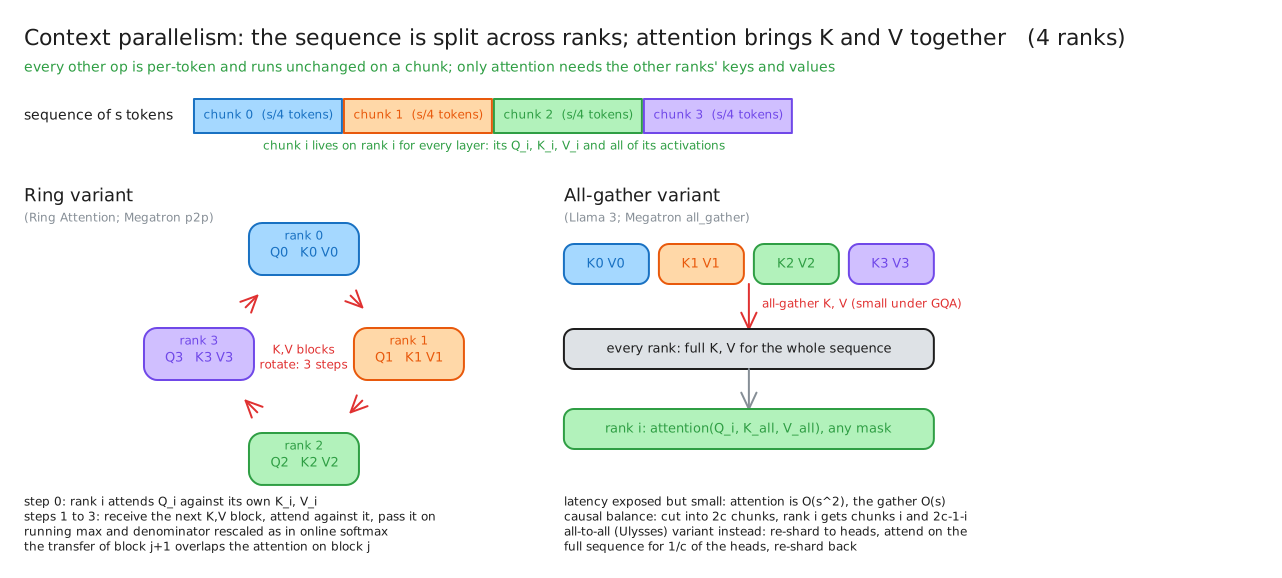
Llama 3’s choice of the all-gather method, with its latency deliberately exposed, is the instructive one, because the report explains the arithmetic (Section 3.3.2). Under grouped-query attention the \(K\) and \(V\) tensors are much smaller than \(Q\) (Llama 3 70B has 8 KV heads against 64 query heads), so the gathered bytes are small; and attention’s compute grows as \(O(s^2)\) while the gather grows as \(O(s)\), so at 128K tokens the gather is a rounding error next to the attention it feeds. Two further details from the same paragraph are worth knowing. First, a causal mask makes the work uneven: the chunk at the end of the sequence attends to everything, the chunk at the start to almost nothing. Llama 3 balances it by cutting the sequence into \(2c\) chunks and giving rank \(i\) chunks \(i\) and \(2c - 1 - i\), one light and one heavy; Megatron Core does the same kind of balancing for its ring implementation. Second, GQA helps CP directly: the Megatron docs note that MQA and GQA reduce the CP communication volume for exactly this reason, only the few KV heads travel.
Where CP sits in the hierarchy follows from its traffic: per layer, like TP, but overlappable or small, unlike TP. Llama 3 places it second, \([\text{TP}, \text{CP}, \text{PP}, \text{DP}]\), and the total GPU count is \(\text{TP} \times \text{CP} \times \text{PP} \times \text{DP}\) (Megatron Core docs).
The naming collision, settled
“Sequence parallelism” is used for both of the previous two ideas, and the collision is a genuine source of confusion:
| Megatron sequence parallelism | Context parallelism | |
|---|---|---|
| Introduced in | Korthikanti et al. 2022 | Li et al. 2021, which calls it “sequence parallelism”; Ring Attention; DeepSpeed-Ulysses, which also calls it sequence parallelism |
| What is split along the sequence | only the norm and dropout activations between TP blocks, within a TP group | the input and every activation, for the whole network |
| Attention | unchanged: each rank has its heads’ full \(K\) and \(V\) | each rank has \(K\) and \(V\) for its own chunk only and needs everyone else’s |
| Purpose | activation memory, at no extra communication | sequences too long for one GPU at all |
When a paper or a flag says “sequence parallel”, check which of the two it means: if it is a companion to tensor parallelism and costs nothing, it is the first; if it is about long context and touches attention, it is the second, and modern frameworks call that one context parallelism.
Expert parallelism: splitting a model that is mostly experts
A mixture-of-experts (MoE) layer replaces the single dense MLP with \(E\) separate MLPs, the experts, and a small router that picks, for each token, the \(k\) experts that token will go through; the token’s output is the gate-weighted sum of those \(k\) experts’ outputs. GShard used top-2 routing (Lepikhin et al.), the Switch Transformer argued for top-1 (Fedus et al.), and DeepSeek-V3 routes each token to 8 of 256 routed experts plus 1 shared expert that every token uses (DeepSeek-V3, Section 4.2). The point of the design is the ratio it creates: compute per token scales with \(k\), parameters scale with \(E\). DeepSeek-V3 has 671B parameters and activates 37B per token.
That ratio is a problem for everything in this post that assumed parameters and FLOPs go together. All 671B parameters must be resident, because any token may route to any expert, so the \(16N\) accounting applies to the full count while the \(6N\) per token applies only to the active slice. And tensor parallelism is a poor fit for experts: each expert is a small MLP (DeepSeek-V3’s have an intermediate width of 2048, against 7168 for the hidden size), so slicing it eight ways produces GEMMs too thin to run efficiently while still paying TP’s collectives; Megatron’s MoE guide recommends an expert tensor-parallel degree of 1 for fine-grained MoE models for exactly this reason (Megatron Core MoE README).
Expert parallelism (EP) is the natural split instead: keep each expert whole and place different experts on different GPUs, \(E / \text{EP}\) per rank. DeepSeek-V3 deploys its 256 routed experts uniformly over 64 GPUs across 8 nodes, four experts per GPU per layer (Section 4.2). The consequence is that tokens have to travel to their experts, and that traffic is the all-to-all from the primitives table:
- Dispatch. After the router decides, every rank sends each of its tokens’ hidden vectors to the ranks hosting that token’s \(k\) experts. Since every rank sends to every other rank, this is one all-to-all.
- Compute. Each rank runs its resident experts on whatever tokens arrived, one grouped or batched GEMM per expert.
- Combine. A second all-to-all sends each expert output back to the token’s home rank, which sums the \(k\) results with the router’s gate weights.
The backward pass mirrors both, so an MoE layer costs two all-to-alls forward and two backward. GShard framed the same movement as an all-to-all resharding on TPUs (Section 3.3.2); Megatron-LM’s --moe-token-dispatcher-type alltoall and the DeepEP-backed dispatcher are the GPU versions, with --expert-model-parallel-size setting the EP degree (MoE README).
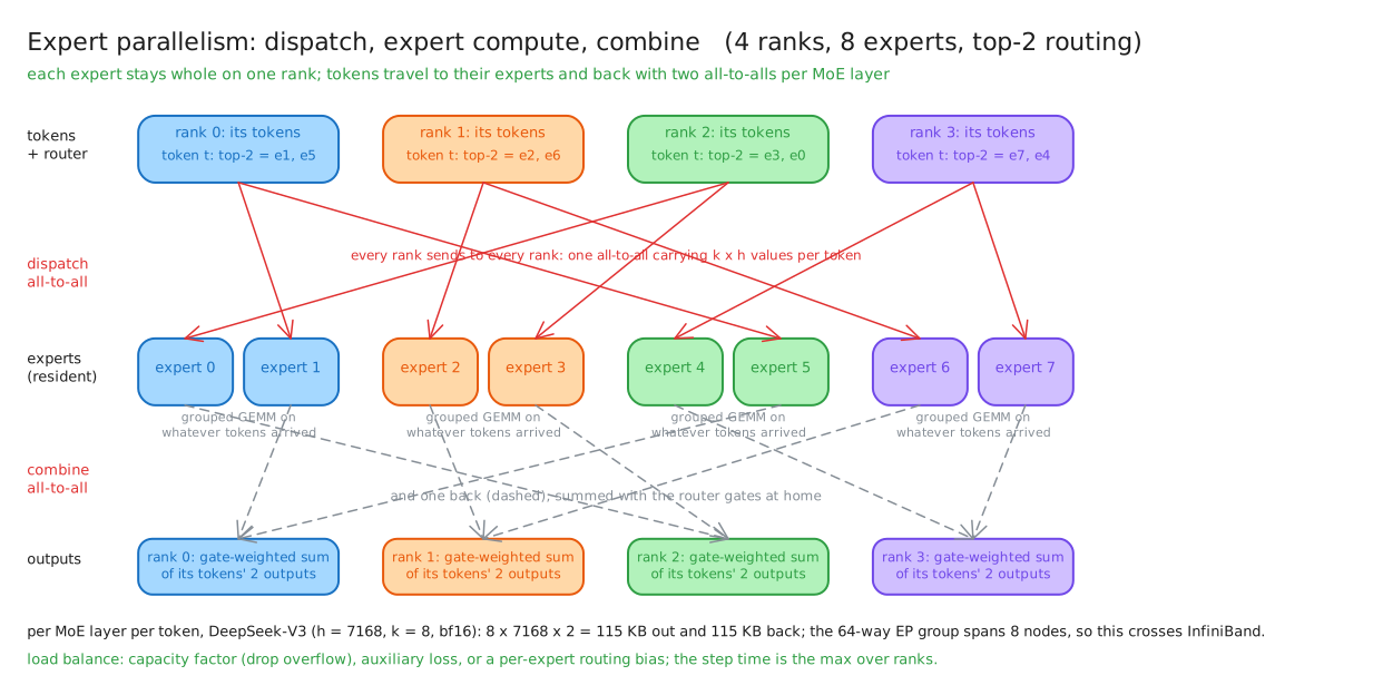
What it costs. Each token’s \(h\)-vector is sent to \(k\) experts and \(k\) results come back, so per MoE layer a rank sends roughly \(2\,k\,b\,s\,h\) bytes-per-element, less whatever fraction of experts happen to be local. For DeepSeek-V3, \(h = 7168\) and \(k = 8\) in bf16 is \(8 \times 7168 \times 2 = 115\) KB per token per layer each way, and there are 58 MoE layers (61 layers with the first three dense). Compare tensor parallelism’s four all-reduces at \(t = 8\), \(16 \times 7168 \times 2 \times 7/8 = 200\) KB per token per layer: the same order of magnitude, but EP’s traffic crosses nodes, since 64 experts’ worth of GPUs do not fit in one. The report is candid about the result: cross-node expert parallelism gave a compute-to-communication ratio of about 1:1 (Section 3.2.1), which is why the two engineering investments of that run, DualPipe’s overlap of a forward chunk’s dispatch and combine with a backward chunk’s compute, and custom all-to-all kernels, both exist. Two tricks in those kernels are worth knowing because they are the bandwidth ladder applied to routing (Section 3.2.2): node-limited routing caps each token at 4 destination nodes so that InfiniBand carries at most 4 copies of it, and each copy is sent once over InfiniBand to a same-index GPU on the target node and then forwarded over NVLink (160 GB/s on their H800 nodes against 50 GB/s for InfiniBand) to the GPUs that actually host the experts. With that structure a token could reach 13 experts for the same cross-node cost as its 8.
Load balance. A synchronous step ends when the busiest GPU finishes, so if the router sends 30% of tokens to one expert, the GPU hosting it becomes the straggler for every step. Three families of remedy:
| Remedy | Mechanism | Where |
|---|---|---|
| Expert capacity | cap the tokens an expert may take per batch at \((\text{tokens}/E) \times\) a capacity factor; overflow tokens skip the layer (Switch reports typically under 1% dropped at factor 1.0 to 1.25) | GShard, Switch Transformer; Megatron --moe-expert-capacity-factor |
| Auxiliary loss | add a differentiable loss that penalizes uneven routing, with a small coefficient (Switch uses \(10^{-2}\)) | same; Megatron --moe-router-load-balancing-type aux_loss |
| Auxiliary-loss-free | add a per-expert bias to the routing score used for top-\(k\) selection only, and nudge it up or down after each step depending on whether the expert was under- or over-loaded; the gate weights themselves are untouched, so the loss is not distorted | DeepSeek-V3, Section 2.1.2, bias update rate \(10^{-3}\); Megatron --moe-router-enable-expert-bias |
Megatron also supports “dropless” MoE, where no token is ever discarded and the expert GEMMs are sized to whatever arrives, at the cost of dynamic shapes.
How EP composes. The older constraint was \(\text{EP} \leq \text{DP}\): an expert-parallel group was carved out of a data-parallel group, since the attention layers on those ranks are replicas of each other while their experts are different. Megatron Core’s “parallel folding” removes that coupling by giving the attention layers and the MoE layers separate parallelism layouts, \(\text{TP} \times \text{CP} \times \text{DP} \times \text{PP}\) for attention and \(\text{ETP} \times \text{EP} \times \text{EDP} \times \text{PP}\) for the experts, so that a run can use high TP and CP where attention wants them and high EP with no TP where the experts want it (MoE README). DeepSeek-V3 is the existence proof of the shape this produces: 16-way pipeline parallelism, 64-way expert parallelism across 8 nodes, ZeRO-1 data parallelism, and no tensor parallelism at all (Section 3.2). The ordering rule survives, but the dimension on the fast link changes with the model: for a dense model it is TP, for a fine-grained MoE it is the expert all-to-all.
The three, side by side
| Sequence parallelism | Context parallelism | Expert parallelism | |
|---|---|---|---|
| Group | the TP group | a CP group, inside the PP stage | an EP group, usually spanning nodes |
| What each rank holds | \(s/t\) tokens of the norm and dropout activations, full tokens elsewhere | \(s/c\) tokens of everything | \(E/\text{EP}\) whole experts, all tokens’ attention |
| Collectives per layer | all-gather and reduce-scatter at each TP boundary | ring point-to-point, all-gather, or all-to-all, in attention only | two all-to-alls forward, two backward |
| Memory effect | activations \(\div t\) across the whole layer | activations \(\div c\), including the attention scores | parameters \(\div \text{EP}\) for the experts |
| Turn it on when | always, with TP | the sequence is too long for one rank | the model is a mixture of experts |
References
- Reducing Activation Recomputation in Large Transformer Models - Korthikanti et al.
- Sequence Parallelism: Long Sequence Training from System Perspective - Li et al., Ring Attention with Blockwise Transformers - Liu et al., DeepSpeed-Ulysses - Jacobs et al.
- Megatron Core context parallelism, Megatron Core MoE README, Megatron-LM arguments
- GShard - Lepikhin et al., Switch Transformers - Fedus et al.
- DeepSeek-V3 Technical Report
- The Llama 3 Herd of Models
Pipeline Parallelism
Tensor parallelism splits every layer across GPUs. Pipeline parallelism (PP) splits the stack of layers: with \(p\) stages, stage 1 holds the first \(L/p\) layers, stage 2 the next \(L/p\), and so on, each stage on its own GPU (or its own tensor-parallel group of GPUs). Data flows through the stages the way it flows through the layers: stage \(i\) runs its layers on an input and sends the output activation to stage \(i+1\); in the backward pass, gradients flow the other way.
Why the communication is cheap
The only thing crossing a stage boundary is the hidden state at that point in the network: one \(b \times s \times h\) tensor forward and its gradient backward, per microbatch, sent point-to-point from one GPU to one other (Narayanan et al., Section 3.2; GPipe makes the same point, that only activations at partition boundaries need to move, Section 2.3). Compare that with tensor parallelism, which all-reduces a tensor of the same size four times per layer. Pipeline parallelism pays once per stage, however many layers the stage contains, and it pays with a single send rather than a collective. In the 70B example, TP moved 75 GB per rank per microbatch; a 16-stage pipeline moves one 134 MB activation per boundary, and can do it asynchronously while the stage works on the next microbatch. That difference in volume is why pipeline parallelism is the split that goes across nodes, on the slow link.
Microbatches and the bubble
The problem with a pipeline is that a naive one is almost entirely idle. If the whole batch went through stage 1, then stage 2, and so on, only one stage would ever be working. So the batch is cut into \(m\) microbatches, and the stages work on different microbatches at the same time: stage 1 finishes microbatch 1 and hands it to stage 2, then starts on microbatch 2 while stage 2 works on microbatch 1, and so on. In steady state every stage is busy on a different microbatch.
The waste is at the ends. Let \(t_f\) and \(t_b\) be the time for one stage to run the forward and backward pass of one microbatch. The ideal time for the batch, with every stage always busy, would be \(m(t_f + t_b)\). But at the start, stage \(p\) cannot begin until microbatch 1 has traversed the \(p - 1\) stages before it, and at the end, stage 1 cannot finish its backward work until the last microbatch’s gradient has come back through the \(p - 1\) stages after it. Fill and drain together idle each stage for \((p-1)(t_f + t_b)\), the pipeline bubble, and its size relative to the useful work is (Narayanan et al., Section 2.2.1):
\[\frac{t_{\text{bubble}}}{t_{\text{ideal}}} = \frac{(p-1)(t_f + t_b)}{m\,(t_f + t_b)} = \frac{p-1}{m}\]Two forms of this are in circulation and both are right; they differ in the denominator. Megatron’s \((p-1)/m\) is bubble over ideal time, the overhead. GPipe’s \(O\!\left(\frac{K-1}{M+K-1}\right)\) (Section 2.3, with \(K\) stages and \(M\) microbatches) is bubble over total time, the idle fraction. Evaluating both:
| \(p\) stages | \(m\) microbatches | Overhead \((p-1)/m\) | Idle fraction \((p-1)/(m+p-1)\) |
|---|---|---|---|
| 8 | 8 | 87.5% | 46.7% |
| 8 | 32 | 21.9% | 17.9% |
| 8 | 64 | 10.9% | 9.9% |
| 16 | 64 | 23.4% | 19.0% |
The rule that falls out is \(m \gg p\): GPipe found the overhead negligible once \(M \geq 4K\), and Megatron’s later work chases the bubble further still. Since the microbatches of the pipeline are the microbatches of gradient accumulation, \(m\) is bounded above by the global batch: \(m = \text{batch per data-parallel rank} / \text{microbatch size}\), so a larger pipeline needs a larger batch to keep its bubble small, which is one of the pressures toward the 16M-token batches large runs use.
Schedules
The bubble fraction is the same for every schedule below; what differs is how many microbatches’ activations are alive at once, which is what decides whether the run fits.
GPipe (Huang et al.) runs all \(m\) forwards, then all \(m\) backwards. Simple, but every microbatch’s activations are stashed until its backward pass arrives, so activation memory scales with \(m\), which directly fights the \(m \gg p\) rule.
1F1B, one-forward-one-backward, comes from PipeDream (Narayanan et al. 2019, Section 3.3), which coined the term. After a warm-up in which each stage runs a few forwards, every stage alternates: one forward on a new microbatch, one backward on an old one. A backward pass frees that microbatch’s activations, so at most \(p\) microbatches are in flight at any moment, and memory scales with \(p\) instead of \(m\). PipeDream itself was asynchronous (it kept multiple weight versions to avoid ever flushing the pipeline). The synchronous variant, PipeDream-Flush (Narayanan et al. 2020, Section 3.2), keeps the 1F1B order, uses a single weight version, and flushes the pipeline at the end of each batch for the optimizer step. That is the schedule Megatron-LM uses by default (Section 2.2.1): same bubble as GPipe, activation memory of \(p\) microbatches instead of \(m\). It is strictly better, and it is the baseline everything else improves on.
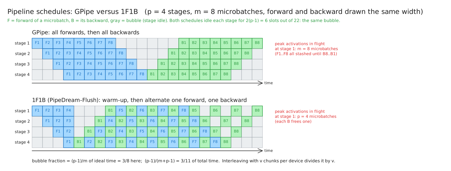
One consequence of 1F1B worth knowing: the memory is uneven across stages. Stage 1 must hold activations for \(p\) microbatches while the last stage holds only 1. With \(L/p\) layers per stage, the first stage’s \(p\) in-flight microbatches add up to a full \(L\) layers’ worth of activations, which is why the activation-memory analyses quote the first stage as the binding constraint (Korthikanti et al., Section 4.2.3).
Interleaved 1F1B (Narayanan et al. 2021, Section 2.2.2) shrinks the bubble itself. Instead of one contiguous block of layers, give each device \(v\) smaller, non-adjacent chunks (with 16 layers and 4 devices, device 1 gets layers 1-2 and 9-10 rather than 1-4). Each chunk’s forward and backward is \(v\) times shorter, so the fill and drain are \(v\) times shorter, and the bubble becomes:
\[\frac{1}{v}\cdot\frac{p-1}{m}\]The cost is that each microbatch now crosses \(v\) times as many stage boundaries, so point-to-point communication goes up by \(v\), and \(m\) must be a multiple of \(p\). This is the schedule Llama 3 trains with, and its report writes the bubble in exactly this form, \((\text{PP}-1)/(V \cdot M)\) (Section 3.3.2).
Zero-bubble schedules attack the last of it with the observation from the very first section: the backward pass is two matmuls, \(\partial L / \partial z = A^\top g\) and \(\partial L / \partial A = g z^\top\), and they have different urgency. The input gradient is on the critical path, since the previous stage is waiting for it. The weight gradient is needed only by the optimizer step at the end of the batch. So split the backward into \(B\) (input gradient) and \(W\) (weight gradient) and schedule \(W\) into the bubbles (Qi et al.). Their ZB-H1 schedule cuts the bubble to a third of 1F1B’s at the same memory; ZB-H2 eliminates it entirely at the cost of more activations in flight. The one obstacle is the optimizer step’s own synchronization (the global gradient-norm for clipping is an all-reduce across stages that would stall the pipeline), which they replace with a post-hoc validation and a rollback if it fails. DeepSeek-V3’s DualPipe goes further, feeding microbatches from both ends of the pipeline and overlapping each forward chunk with a backward chunk’s compute and communication; its bubble is \((\text{PP}/2 - 1)(F\&B + B - 3W)\) against 1F1B’s \((\text{PP}-1)(F+B)\), paid for with two copies of the parameters (DeepSeek-V3, Section 3.2.1 and Table 2).
Whether you need these depends on where the bubble sits in your budget. With \(p = 16\), \(v = 8\), \(m = 32\), the interleaved bubble is \(15/256 \approx 6\%\); zero-bubble buys back that last few percent. For most runs the useful hierarchy is: 1F1B as the baseline, interleaving when \(p\) is large, zero-bubble when the last percent is worth the complexity.
Why pipeline parallelism is awkward for inference
In training there are \(m\) microbatches to fill the pipe, and \(m\) is under your control. In decode there is one token per sequence per step, so a request has nothing with which to fill the stages behind it; the only “microbatches” are other concurrent requests, and the pipeline sits in its bubble whenever there are too few of them. That is why serving keeps tensor parallelism within a node and scales out with data-parallel replicas, and treats pipeline parallelism as a fit-the-model tool rather than a throughput tool (the inference post covers that side).
References
- Efficient Large-Scale Language Model Training on GPU Clusters Using Megatron-LM - Narayanan et al.
- GPipe - Huang et al.
- PipeDream: Generalized Pipeline Parallelism for DNN Training - Narayanan et al., Memory-Efficient Pipeline-Parallel DNN Training (PipeDream-Flush and 2BW) - Narayanan et al.
- Zero Bubble Pipeline Parallelism - Qi et al.
- DeepSeek-V3 Technical Report
- Reducing Activation Recomputation in Large Transformer Models - Korthikanti et al.
- The Llama 3 Herd of Models
Composing Them: 3D and 4D Parallelism
No single dimension gets a large model trained. Tensor parallelism cannot leave the node, pipeline parallelism wastes a bubble per stage, and data parallelism does nothing for a model that does not fit. Real runs use all of them at once, and the number of GPUs is their product:
\[\text{GPUs} = \text{TP} \times \text{CP} \times \text{PP} \times \text{DP}\](times an expert-parallel degree for mixture-of-experts models). The question is which dimension goes where in the hardware, and the previous sections have already answered it, one dimension at a time.
The ordering rule
Put the four dimensions’ communication side by side, per microbatch unless stated:
| Dimension | What it moves | How often | Can it hide behind compute? |
|---|---|---|---|
| TP | 4 all-reduces of the \(b \times s \times h\) hidden state | per layer | barely; each sits between two dependent matmuls |
| CP | \(K\) and \(V\) blocks around a ring | per layer, attention only | yes, by design, behind block-wise attention |
| PP | one \(b \times s \times h\) activation (and its gradient), point to point | per stage boundary | yes, asynchronously, behind the next microbatch |
| DP | the gradient reduce, plus the parameter gather if sharded: \(2\Psi\) to \(3\Psi\) elements | once per step | yes, behind the backward pass (and the next forward, for prefetched gathers) |
Reading down the rows, the traffic gets less frequent and more overlappable, and that ordering is the placement rule: the chattiest dimension goes on the fastest link. TP on NVLink inside a node, PP across nodes on the network, DP outermost on whatever is left, with CP slotted between TP and PP when it is in use. Llama 3 states the rule and the order explicitly: the innermost parallelism needs the highest bandwidth and lowest latency and is kept within a server, so they place the dimensions in the order \([\text{TP}, \text{CP}, \text{PP}, \text{DP}]\), with DP outermost because it tolerates the network’s latency thanks to asynchronous prefetching of weights and reduction of gradients (Section 3.3.2). Megatron’s guidelines say the same in two takeaways: use tensor parallelism up to the number of GPUs in a server, then pipeline parallelism to scale across servers (Narayanan et al., Section 3.2).
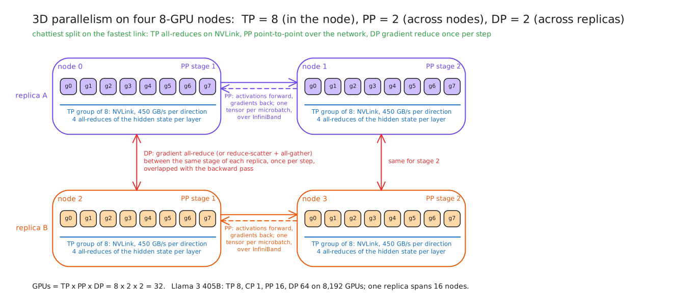
What a real run looks like
Llama 3’s report gives the actual configurations of its 405B pre-training, which is rare and worth studying line by line (Table 4):
| GPUs | TP | CP | PP | DP | Seq. len. | Batch per DP rank | Tokens per batch | TFLOPs per GPU | BF16 MFU |
|---|---|---|---|---|---|---|---|---|---|
| 8,192 | 8 | 1 | 16 | 64 | 8,192 | 32 | 16M | 430 | 43% |
| 16,384 | 8 | 1 | 16 | 128 | 8,192 | 16 | 16M | 400 | 41% |
| 16,384 | 8 | 16 | 16 | 8 | 131,072 | 16 | 16M | 380 | 38% |
Check the arithmetic and the rule against it. \(8 \times 1 \times 16 \times 64 = 8{,}192\) and \(8 \times 16 \times 16 \times 8 = 16{,}384\), as required. TP is 8, the size of a node, in every row: it never leaves NVLink. PP is 16 in every row, so one model replica spans \(8 \times 16 = 128\) GPUs, sixteen nodes, and everything beyond that is DP. When the sequence length goes to 128K, CP goes to 16, and since the GPU count is fixed, DP drops from 128 to 8 to make room. Tokens per batch stay at 16M throughout: in the first row that is \(64 \times 32 \times 8{,}192 = 16.8\)M, in the third \(8 \times 16 \times 131{,}072 = 16.8\)M. And the utilization drifts down as DP grows, which the report attributes to the smaller batch per DP rank needed to keep the token count fixed: fewer microbatches per pipeline, a larger bubble.
The per-GPU memory picture at this scale is instructive. One replica holds the 405B model over 128 GPUs, so the bf16 weights are \(810 / 128 \approx 6.3\) GB per GPU, and the remaining 14 bytes per parameter, sharded by FSDP across the 64 or 128 data-parallel ranks as well, are under a gigabyte. Static state, the thing that dominated the single-GPU discussion, has become small; what fills the 80 GB now is activations for the \(p\) microbatches a 1F1B stage keeps in flight, plus the communication buffers. At scale the memory problem turns into a scheduling problem.
How to choose
The Megatron paper’s guidelines, restated as a procedure (Section 3):
- Tensor parallelism up to the node, and no further. Use as little as makes the per-GPU slice of weights and activations fit, since each doubling thins the per-rank GEMMs and adds collectives; in practice 8 for large models.
- Pipeline parallelism just large enough that, with TP, the model fits. Every extra stage adds bubble, so the model-parallel product \(\text{TP} \times \text{PP}\) should be the smallest that fits the parameters and activations.
- Everything else to data parallelism. It scales best, because its one collective per step hides behind the backward pass.
- Then tune the microbatch and \(m\). Raise the number of microbatches until the bubble is a few percent, and set the microbatch size as large as memory allows so the GEMMs are efficient; the global batch follows as \(\text{DP} \times \text{microbatch} \times m\).
Context parallelism enters when the sequence length forces it, and expert parallelism when the model is a mixture of experts, as the previous section laid out; the DeepSeek-V3 layout of \(\text{PP} = 16\) and \(\text{EP} = 64\) across 8 nodes with no tensor parallelism (Section 3.2) is what the same procedure produces when the expert all-to-all, not the TP all-reduce, is the traffic that needs the fast link.
References
- The Llama 3 Herd of Models
- Efficient Large-Scale Language Model Training on GPU Clusters Using Megatron-LM - Narayanan et al.
- DeepSeek-V3 Technical Report
MFU and HFU
Everything above is in service of one number, and it is the one leadership asks about: what fraction of the hardware’s peak arithmetic is the run actually using.
The definition, and why tokens per second is in it
Model FLOPs utilization (MFU) was defined by the PaLM paper as the ratio of the observed throughput, in tokens per second, to the theoretical maximum throughput the system could reach at its peak FLOP rate (Chowdhery et al., Section 4.1). The theoretical maximum is easy to write down, because the FLOPs per token are a constant of the model: \(6N\) for the forward and backward pass. So:
\[\text{max tokens/s} = \frac{\text{GPUs} \times \text{peak FLOP/s per GPU}}{6N} \qquad\Longrightarrow\qquad \text{MFU} = \frac{6N \times \text{tokens/s}}{\text{GPUs} \times \text{peak FLOP/s per GPU}}\]Tokens per second appears because it is the thing you can measure: a training loop knows how many tokens it consumed and how long it took. The FLOPs it did are not observed, they are inferred, by multiplying the token rate by the model’s fixed cost per token. The numerator is therefore “the FLOPs the model needed”, counted from the token rate, and the denominator is “the FLOPs the hardware could have done”. PaLM’s Appendix B adds the attention term to the numerator, \(6N + 12\,L\,H\,Q\,T\) per token with \(L\) layers, \(H\) heads, \(Q\) head dimension, and \(T\) sequence length; for PaLM it moved the answer from 45.7% to 46.2%, and it grows with \(T\).
Hardware FLOPs utilization (HFU) is the other number, and the distinction matters: HFU counts every FLOP the hardware executed, including the recomputation from activation checkpointing, against peak. MFU counts only the FLOPs the model needed. So \(\text{HFU} \geq \text{MFU}\) always, with equality when nothing is recomputed, and the gap is the recompute tax made visible. PaLM ran with full recomputation and reported 46.2% MFU against 57.8% HFU; Megatron’s selective-recompute 1T run reported 56.3% MFU against 57.0% HFU (Korthikanti et al., Table 5), a gap of under one point. Quoting HFU when the question was MFU inflates the answer by exactly the amount of work that was not useful, and PaLM’s paper points out that earlier reports, including Megatron’s 52%, were computed the hardware way.
Both directions, worked
Measured to MFU. Llama 3’s second configuration reports 400 TFLOPs per GPU, and dense BF16 peak is about 989 TFLOPS, so \(400 / 989 = 40.4\%\) against the report’s 41% (its TFLOPs figure is itself rounded) (Table 4); the first row’s 430 gives 43%. Now go through tokens instead. At 400 TFLOPs on 16,384 GPUs the run does \(6.55 \times 10^{18}\) useful FLOP/s, and a 405B model costs \(6 \times 405 \times 10^9 = 2.43 \times 10^{12}\) FLOPs per token, so:
\[\text{tokens/s} = \frac{6.55 \times 10^{18}}{2.43 \times 10^{12}} \approx 2.7 \times 10^{6}\]A 16.8M-token batch is then about 6.2 s per step, and the paper’s 15.6T pre-training tokens would take \(15.6 \times 10^{12} / 2.7 \times 10^{6} \approx 5.8 \times 10^{6}\) s, about 67 days of step time at that stage’s rate (the actual run also had a long-context stage at lower MFU and a ramp-up at smaller batch, so this is the order of magnitude, not the schedule).
MFU to expected throughput. Suppose a 70B model on 1,024 H100s reports 12,000 tokens/s. Then \(6 \times 70 \times 10^9 \times 12{,}000 = 5.0 \times 10^{15}\) FLOP/s achieved, against \(1{,}024 \times 989 \times 10^{12} = 1.0 \times 10^{18}\) peak: an MFU of 0.5%. Nothing is that bad by accident; something is broken. Running it the other way says what to expect: at 40% MFU those GPUs should deliver \(0.4 \times 1.0 \times 10^{18} / (4.2 \times 10^{11}) \approx 965{,}000\) tokens/s, eighty times more. Being able to do this estimate in both directions from three numbers, model size, GPU count, token rate, is the fastest sanity check there is on any training run.
Reference points
Published, verified figures, so you know what “good” looks like:
| Run | Scale | Utilization | Source |
|---|---|---|---|
| GPT-3 175B | 21.3% MFU (as computed by PaLM) | PaLM, Table 3 | |
| Gopher 280B | 32.5% MFU | same | |
| Megatron-Turing NLG 530B | 30.2% MFU | same | |
| Megatron 1T GPT | 3,072 A100 | 52% of peak, hardware FLOPs | Narayanan et al. |
| PaLM 540B | 6,144 TPU v4 | 46.2% MFU, 57.8% HFU | PaLM, Section 4.1 |
| Megatron 530B with selective recompute and SP | 2,240 A100 | 54.2% MFU | Korthikanti et al. |
| MegaScale 175B | 12,288 GPUs | 55.2% MFU | Jiang et al. |
| Llama 3 405B | 8,192 to 16,384 H100 | 38 to 43% BF16 MFU | Llama 3, Table 4 |
| Megatron-LM on H100 clusters | up to 47% MFU | Megatron-LM README |
The band for a well-tuned large dense run is roughly 40 to 55% MFU, and it has moved up over time as recomputation got selective and communication got overlapped. Where the rest goes, in the order you would check:
| Loss | Why it shows up | Section |
|---|---|---|
| Exposed communication | collectives not overlapped; TP on the wrong link; too little compute per collective | primitives, data and tensor parallelism |
| Pipeline bubble | \(m\) too small relative to \(p\) | pipeline parallelism |
| Thin GEMMs | microbatch too small for the tensor cores to reach peak; TP degree too high | recomputation, tensor parallelism |
| Recomputation | the HFU-to-MFU gap; full instead of selective | recomputation |
| Stragglers and stalls | one slow rank, or a starved dataloader, idling every collective | what breaks |
| Kernel inefficiency | attention or norm kernels far from roofline | the FlashAttention worklog |
| Wrong peak in the denominator | the “with sparsity” TFLOPS number | the numbers section |
References
- PaLM: Scaling Language Modeling with Pathways - Chowdhery et al.
- Reducing Activation Recomputation in Large Transformer Models - Korthikanti et al.
- Efficient Large-Scale Language Model Training on GPU Clusters Using Megatron-LM - Narayanan et al.
- MegaScale: Scaling Large Language Model Training to More Than 10,000 GPUs - Jiang et al.
- The Llama 3 Herd of Models, Megatron-LM README
What Breaks at Scale
A short section, because the mechanisms are simple even though the engineering is not. The numbers are Llama 3’s, from the most detailed public account of a large run’s operations (Section 3.3.4).
Failures are routine, not exceptional. In a 54-day snapshot of 405B pre-training on 16K GPUs, Llama 3 saw 466 job interruptions, 47 planned and 419 unexpected. About 78% of the unexpected ones were attributed to confirmed or suspected hardware, and GPU problems alone were 58.7% of them (faulty GPUs 30.1%, HBM3 failures 17.2%). That is roughly eight unexpected interruptions per day. The run still achieved over 90% effective training time, which was possible only because restarts were automatic; the paper says manual intervention was needed just three times. Everything below is in service of making an interruption cheap.
Stragglers. A synchronous step ends when its slowest participant finishes, so one GPU that is thermally throttling, or one link with errors, slows every collective it is part of and therefore every GPU in the job. The failure is silent, since nothing crashes; detection is by per-rank timing, and Llama 3 built tooling that prioritizes suspect communications from selected process groups to find slow-but-functioning ranks.
Checkpoints. A checkpoint of the full training state is the 16 bytes per parameter again: about 1.12 TB for a 70B model, 6.5 TB for the 405B. Written synchronously from every rank, that stalls the run for as long as the write takes. Llama 3’s storage tier sustained 2 TB/s with a 7 TB/s peak, sized precisely so that checkpoints could be written quickly enough to be frequent; each GPU’s share is 1 MB to 4 GB depending on the model, and it is written sharded, one piece per rank, rather than gathered (Section 3.3.1). The frequency is set by the interruption rate: with eight interruptions a day, an hour between checkpoints costs an average of half an hour of lost work per interruption.
Loss spikes. Large runs occasionally see the loss jump and sometimes fail to recover. PaLM reports about 20 such spikes, despite gradient clipping, and its remedy is the standard one: restart from a checkpoint roughly 100 steps before the spike and skip 200 to 500 data batches, after which the spike did not recur; they verified the same batches did not spike from a different checkpoint, so it was the combination of data and state, not bad data alone (PaLM, Section 5.1). The everyday defenses are gradient clipping by global norm (Pascanu et al.) and, under fp16, the loss scaler’s skip-on-overflow.
Nondeterminism. Two runs of the same job with the same seed are not bit-identical, and the usual explanation, floating-point addition is not associative and reductions run in parallel, is only half of it. The reduction order changes with the batch composition and the communication topology: a kernel that reduces over a different tile pattern for a different batch size produces different bits, so the same sequence gets a different result depending on what else is in the batch. The Thinking Machines write-up on inference makes this precise as a lack of batch invariance in the kernels, and shows it by getting 80 distinct completions from 1,000 greedy runs of the same prompt (Defeating Nondeterminism in LLM Inference). In training this is usually harmless, but it matters when a divergence has to be reproduced to be debugged, and it is the same class of issue that showed up in the EAGLE data-parallel test. Determinism is buyable, at a cost in kernel choice and speed.
The dataloader. Trivially overlooked and a common reason a run sits at half the MFU it should: if the input pipeline (reading, tokenizing, packing, shipping to the GPU) cannot keep up with the step time, every step waits on it, and the GPU profile shows idle time at the start of each step that no parallelism setting will fix. It is the first thing to rule out when MFU is low and the collectives look healthy.
References
- The Llama 3 Herd of Models
- PaLM: Scaling Language Modeling with Pathways - Chowdhery et al.
- On the difficulty of training Recurrent Neural Networks - Pascanu et al.
- Defeating Nondeterminism in LLM Inference - Thinking Machines
Takeaways
The things worth carrying out of this post, each one traceable to a section above:
- \(6N\) for training, \(2N\) for inference. The backward pass is two matmuls per weight, the outer product \(g z^\top\) for the weights and \(A^\top g\) for the input, each a forward’s worth of work. The weight gradient is why activations must be saved.
- 16 bytes per parameter for bf16 with Adam: 2 weights, 2 gradients, 4 master weights, 4 and 4 for the moments. Static state scales with \(N\) only; an 8B model’s state does not fit on an 80 GB GPU. This is the number that motivates ZeRO, FSDP, and model parallelism.
- Master weights are fp32 because a bf16 weight cannot absorb an update below about \(2^{-8}\) of its own size; the update rounds to nothing. fp32 pushes that floor to \(2^{-24}\).
- bf16 trades mantissa for exponent and needs no loss scaling; fp16 needs it because its gradients underflow. FP8 uses E4M3 forward and E5M2 for gradients, needs scaling factors, and accumulates in fp32.
- Activations scale with \(b \times s \times L\), and per layer they are \(sbh(34 + 5as/h)\). The quadratic term is the attention scores, and selective recomputation (or a fused attention kernel) removes it for a few percent of FLOPs; full recomputation costs a third.
- A ring all-reduce costs each rank \(2S(p-1)/p\), because it is a reduce-scatter plus an all-gather, each moving the \(p-1\) chunks a rank does not already own. That identity is what ZeRO’s sharded optimizer step exploits, and the \((p-1)/p\) is why the cost is flat in \(p\).
- ZeRO 1, 2, 3 shard optimizer state, gradients, and parameters, for \(4 + 12/D\), \(2 + 14/D\), and \(16/D\) bytes per parameter. Stages 1 and 2 cost no extra communication; stage 3 costs \(1.5\times\) for the second parameter gather, and FSDP hides it by prefetching the next layer’s gather behind the current layer’s compute.
- Gradient accumulation sums \(k\) microbatch gradients before one optimizer step: activations of one microbatch at a time, the collective once per step, and under pipeline parallelism the same microbatches fill the pipe.
- Tensor parallelism splits column-then-row so the nonlinearity needs no sync, costs four all-reduces per layer on the critical path, and stays inside the node.
- Sequence parallelism splits the norm and dropout regions along the sequence for the same communication and less memory. Context parallelism splits the sequence itself and brings keys and values together by ring, all-gather, or all-to-all. Expert parallelism keeps each expert whole on one GPU and moves tokens to experts with a dispatch and a combine all-to-all, which becomes the dominant traffic in MoE training.
- The pipeline bubble is \((p-1)/m\) of ideal time. 1F1B keeps it with \(p\) microbatches in flight instead of GPipe’s \(m\); interleaving divides it by \(v\); zero-bubble schedules fill it with deferred weight-gradient work.
- Chattiest on the fastest link: TP on NVLink, then CP, then PP across nodes, then DP outermost. Llama 3 runs \([8, 1, 16, 64]\) on 8,192 GPUs at 43% MFU.
- MFU \(= 6N \cdot \text{tokens/s} / (\text{GPUs} \cdot \text{peak})\), tokens per second because that is what you can measure. HFU also counts recomputation, so it is never lower. Good large dense runs sit around 40 to 55%, and the estimate runs in both directions from three numbers.
- At scale, failures are hourly, and the run survives them with automatic restart, sharded asynchronous checkpoints, and straggler detection.
Test Yourself
Everything above, as questions, grouped the way the sections are. Try each from memory before reading its answer; where a question says numbers, do the arithmetic. Every answer traces back to a section and its references.
Shape and memory
1. Why \(6N\) per token for training and \(2N\) for inference? Name the two backward matmuls and their shapes. Forward is \(2N\): two FLOPs per parameter per token. Backward computes, per weight matrix, the weight gradient \(\partial L/\partial A = g z^\top\) (an outer product, \(m \times n\)) and the input gradient \(\partial L/\partial z = A^\top g\) (a transposed matmul, \(n \times 1\)), each the same size multiply as the forward, so \(4N\); total \(6N\). Inference has no backward.
2. Numbers: bytes per parameter for bf16 with Adam, and does an 8B model’s static state fit on one 80 GB H100? 2 (weights) + 2 (gradients) + 4 (fp32 master) + 4 (\(m\)) + 4 (\(v\)) = 16. \(8 \times 10^9 \times 16 = 128\) GB. No, and that is before any activation.
3. Why are master weights fp32? What exactly goes wrong without them? The optimizer update is added to the weight, and bf16 has 7 fraction bits, so any update below about \(2^{-8} \approx 0.4\%\) of the weight rounds away to nothing under round-to-nearest; the update is cancelled, not approximated. fp32’s 23 bits move that floor to \(2^{-24}\).
4. What scales with \(N\), what scales with \(b \times s\), and why does the distinction decide the technique? Static state (weights, gradients, optimizer) scales with \(N\) only, so sharding across ranks or splitting the model fixes it. Activations scale with \(b \times s \times L\), so recomputation, smaller microbatches, and sequence or context parallelism fix them. A real run needs both.
5. Numbers: activation memory for the Llama 3 8B architecture at microbatch 4, sequence 8192, 16-bit, no parallelism, no recomputation. \(h = 4096\), \(a = 32\), \(L = 32\). \(sbh = 8192 \times 4 \times 4096 = 1.34 \times 10^8\); \(5as/h = 5 \times 32 \times 8192 / 4096 = 320\); per layer \(1.34 \times 10^8 \times (34 + 320) = 47.5\) GB; times 32 layers about 1.5 TB. With the score term removed (FlashAttention or selective recompute) the \(34\,sbh\) alone is 4.6 GB per layer, 146 GB total.
Precision
6. fp16 versus bf16: bits, ranges, and which needs loss scaling and why. fp16 is 1/5/10 with a maximum of 65,504 and a smallest normal of \(6.1 \times 10^{-5}\); bf16 is 1/8/7 with fp32’s range. Gradients underflow fp16’s range, so fp16 needs loss scaling; bf16 does not, because the range problem does not exist there.
7. How does dynamic loss scaling work, and what happens on an overflow? Multiply the loss by a scale \(S\) before backward, unscale the gradients before clipping and the update. Start large (\(2^{16}\) in PyTorch), double after 2,000 consecutive clean steps; on an inf or NaN, skip that optimizer step entirely and halve the scale.
8. FP8 E4M3 versus E5M2: which for what, and why does that follow from the bit layout? E4M3 (max 448, 3 fraction bits) for weights and activations, which need precision more than range; E5M2 (max 57,344, 2 fraction bits) for gradients, which need range for the same reason fp16 gradients underflow. Both need per-tensor or per-block scaling because 448 is a tight ceiling.
9. What is delayed scaling and what does it avoid? Choosing the FP8 scale factor from the amax history of previous iterations instead of the current tensor, on the assumption that ranges change slowly; it avoids a full pass over the tensor (and a synchronization) before every cast. DeepSeek-V3 instead scales online per \(1 \times 128\) tile and \(128 \times 128\) block.
10. What stays fp32 no matter what? State the rule, not the list. Reductions and updates in fp32, matmul operands in low precision. Concretely: master weights, the optimizer moments and update, tensor-core accumulators, the loss and gradient-norm reductions, and norm and softmax statistics.
11. Which architecture generation gates bf16, FP8, FP4? bf16 tensor cores from Ampere (A100); FP8 from Ada (compute capability 8.9) and Hopper (9.0), absent on A100; FP4 with hardware block scaling (NVFP4, MXFP4) from Blackwell.
Sharding
12. ZeRO stages 1, 2, 3: what is sharded, memory per GPU, communication relative to DDP. 1: optimizer state, \(4 + 12/D\), same as DDP. 2: plus gradients, \(2 + 14/D\), same. 3: plus parameters, \(16/D\), \(1.5\times\).
13. Why is ZeRO-3 \(1.5\times\) the communication of DDP? Where does the extra half come from? DDP’s all-reduce is a reduce-scatter plus an all-gather, \(2\Psi\). ZeRO-3 must all-gather each layer’s parameters before its forward, free them, and all-gather them again before its backward, plus reduce-scatter the gradients: \(3\Psi\). The extra \(\Psi\) is the second parameter gather.
14. Why is FSDP usable at all given that overhead? Prefetching: the all-gather for layer \(i+1\) is issued while layer \(i\) computes (forward prefetch), and likewise in the backward pass, so the extra gather hides behind compute instead of sitting on the critical path.
15. Numbers: 70B model, 64 GPUs, bf16 with Adam. Static memory per GPU under DDP, ZeRO-1, 2, 3, and which fit in 80 GB? DDP \(16 \times 70 = 1{,}120\) GB; ZeRO-1 \((4 + 12/64) \times 70 = 293\) GB; ZeRO-2 \((2 + 14/64) \times 70 = 155\) GB; ZeRO-3 \(70 \times 16 / 64 = 17.5\) GB. Only ZeRO-3 fits; stages 1 and 2 are capped by the replicated 4 and 2 bytes.
16. What does gradient accumulation buy, and what must you do in DDP or FSDP for it to actually save communication? The gradient of a mean is the mean of the gradients, so \(k\) microbatch backward passes summed into one buffer give the gradient of a \(k\) times larger batch with one microbatch’s activations alive at a time. Wrap the first \(k-1\) in no_sync() so the all-reduce (DDP) or reduce-scatter (FSDP) runs once per step; in FSDP that keeps unsharded gradients on every rank meanwhile.
17. When is ZeRO-Offload the right call, and when is it wrong? Right when the run is capacity-bound with wall-clock to spare (few GPUs, large model). Wrong when it is already communication-bound, since it puts PCIe at 64 GB/s per direction, the slowest link in the machine, on the critical path.
Tensor and pipeline parallelism
18. For \(Y = \mathrm{GeLU}(XA)B\), why is \(A\) split by columns and \(B\) by rows? What breaks the other way? A column split of \(A\) gives each rank whole output columns, and GeLU is elementwise, so it applies locally with no sync. A row split would produce partial sums \(X_1A_1 + X_2A_2\) that must be added before the GeLU, since GeLU of a sum is not the sum of GeLUs. \(B\) is then split by rows because its contraction dimension is the one already sharded; the partial \(Y_i\) are summed by one all-reduce at the end.
19. Numbers: all-reduces per transformer layer under TP, and the bytes for \(h = 8192\), 8192 tokens, bf16, \(t = 8\); time on NVLink versus PCIe. Four per layer: two forward (\(g\) after attention and after the MLP), two backward (\(f\)). One hidden state is \(8192 \times 8192 \times 2 = 134\) MB; per all-reduce per rank \(2 \times 134 \times 7/8 = 235\) MB; per layer 0.94 GB; over 80 layers 75 GB per microbatch per rank. At 450 GB/s per direction (NVLink) 0.17 s; at 64 GB/s (PCIe Gen5) 1.2 s; against roughly 1.1 s of compute at 40% MFU.
20. What does sequence parallelism add, and what is its exact benefit? It splits the norm and dropout regions, which TP replicates on every rank, along the sequence, and converts the all-reduce at each TP boundary into a reduce-scatter plus an all-gather. Same communication volume, activation memory divided by \(t\) across the whole layer: the 10 in \(sbh(10 + 24/t + \ldots)\) becomes \(10/t\). It is not a communication reduction.
21. Numbers: derive the pipeline bubble and evaluate for \((p, m) = (8, 8), (8, 64), (16, 64)\). Fill and drain idle each stage for \((p-1)(t_f + t_b)\) against \(m(t_f + t_b)\) of useful work: \((p-1)/m\) of ideal time, or \((p-1)/(m+p-1)\) of total time. \(7/8 = 87.5\%\) (47% of total); \(7/64 = 10.9\%\) (9.9%); \(15/64 = 23.4\%\) (19%).
22. GPipe versus 1F1B: same bubble, different what? Why is 1F1B strictly better? Same bubble fraction, different activation memory: GPipe holds all \(m\) microbatches’ activations until the backward phase, 1F1B holds at most \(p\), because each backward frees a microbatch and the schedule alternates. Since \(m \gg p\) is required for a small bubble, memory that scales with \(p\) instead of \(m\) is strictly better.
23. What does interleaved 1F1B do to the bubble, and what does it cost? With \(v\) non-adjacent layer chunks per device the bubble becomes \((p-1)/(v\,m)\); it costs \(v\) times the point-to-point communication and requires \(m\) to be a multiple of \(p\).
24. Why is PP awkward for inference in a way it is not for training? Training has \(m\) microbatches to fill the pipe, chosen freely. Decode produces one token per sequence per step, so only concurrent requests can act as microbatches; with too few, the pipeline sits in its bubble. Serving uses TP within a node and DP replicas across.
25. The rule for assigning parallelism dimensions to the hardware, in one sentence, with justification. Chattiest on the fastest link: TP does four all-reduces of the hidden state per layer, so NVLink inside the node; PP sends one activation per stage boundary per microbatch, point to point and asynchronous, so across nodes; DP reduces gradients once per step, overlapped with the backward, so outermost. Llama 3’s order is \([\text{TP}, \text{CP}, \text{PP}, \text{DP}]\).
25b. Three ways to do attention under context parallelism, and why Llama 3 chose the one with exposed latency. Ring: pass \(K\) and \(V\) blocks around the CP ring, overlapped with block-wise attention. All-gather: collect all \(K\) and \(V\), then attend locally. All-to-all (Ulysses): re-shard from sequence to heads, attend on full sequences for a subset of heads, re-shard back. Llama 3 uses all-gather because under GQA the gathered \(K\) and \(V\) are small and attention is \(O(s^2)\) against the gather’s \(O(s)\), and because it supports document masks easily.
25c. Why expert parallelism instead of tensor parallelism for a mixture of experts, and what does it communicate? Every expert must be resident since any token may route anywhere, but each expert is a small MLP, so slicing it produces thin GEMMs that still pay TP’s collectives. EP keeps experts whole and places different experts on different ranks; tokens travel to their \(k\) experts and back through a dispatch all-to-all and a combine all-to-all per MoE layer, roughly \(2khb\) bytes per token per layer in bf16, and that traffic crosses nodes.
25d. Three ways to keep expert load balanced. Expert capacity with a capacity factor (overflow tokens skip the layer); an auxiliary load-balancing loss; and DeepSeek-V3’s auxiliary-loss-free bias, added to the routing score for top-\(k\) selection only and nudged after each step.
Collectives and utilization
26. Ring all-reduce volume per rank, and why is all-reduce exactly twice reduce-scatter? \(2S(p-1)/p\). The ring does a reduce-scatter (each rank ends with one fully summed chunk) and then an all-gather (the chunks circulate), each \(p-1\) steps of \(S/p\) bytes; each phase alone is \(S(p-1)/p\).
27. What is gradient bucketing and in what regime does it help? Fusing many small gradient tensors into one collective of about 25 MiB. It helps in the latency-bound regime, where the per-message \(\alpha\) term dominates because the model has thousands of small tensors.
28. Where does DDP overlap communication with compute? Where does FSDP? DDP launches a bucket’s all-reduce as soon as its gradients are ready, while autograd is still computing earlier layers’ gradients. FSDP prefetches the next unit’s parameter all-gather during the current unit’s forward or backward compute, and reduce-scatters gradients as the backward proceeds.
29. Define MFU and HFU. Which is larger with recomputation on, and why? MFU is the FLOPs the model needed, \(6N\) per token times the token rate, over the hardware’s peak. HFU is every FLOP the hardware executed, recomputation included, over peak. HFU is never smaller, and the gap is the recompute tax; PaLM was 46.2% MFU against 57.8% HFU.
30. Numbers: 1,024 H100s, 70B model, 40% MFU. Tokens per second, and time for \(10^{12}\) tokens? \(0.4 \times 1{,}024 \times 989 \times 10^{12} / (6 \times 70 \times 10^9) \approx 965{,}000\) tokens/s; \(10^{12} / 9.65 \times 10^5 \approx 1.04 \times 10^6\) s, about 12 days of step time.
31. Numbers: you measure 18% MFU. Five candidate causes, in the order you would check. The dataloader (idle at the start of every step); exposed communication (gaps on the compute stream while NICs are busy, TP on the wrong link); the pipeline bubble (\(m\) too small for \(p\)); thin GEMMs (microbatch too small, TP degree too high) or full recomputation instead of selective (check HFU against MFU); a straggler (per-rank step-time histogram). Also confirm the denominator uses the dense, not “with sparsity”, peak.
Operations
32. Why are stragglers so damaging, and how would you detect one? Every synchronous collective finishes when its slowest rank does, so one slow GPU slows all of them, silently. Per-rank step and collective timing, and tooling that flags process groups with suspect communication times.
33. Numbers: checkpoint size for a 70B model with full optimizer state, what it does to cadence, and the fix. \(70 \times 10^9 \times 16 = 1.12\) TB. Written synchronously it stalls the run for the write time, which pushes toward infrequent checkpoints, which raises the cost of every one of the roughly daily hardware interruptions. The fix is sharded (one piece per rank), asynchronous checkpoints to a storage tier fast enough for them to be frequent; Llama 3’s sustained 2 TB/s.
34. Four causes of a loss spike, and a mitigation for each. A pathological data batch (skip it: PaLM restarts 100 steps back and skips 200 to 500 batches); a learning rate too high for the current state (clip by global norm, warm up, decay); fp16 overflow (the loss scaler skips the step and backs off); a bad interaction of state and data (roll back to a checkpoint; PaLM showed the same batches did not spike from a different checkpoint).
35. Why is a large run not bit-reproducible, and when does it matter? Reduction order varies with topology and batch composition, and floating-point addition is not associative, so the same computation yields different bits under a different batch or placement; kernels that are not batch-invariant are the sharpest version of this. It usually does not matter, but it does when reproducing a divergence to debug it or when promising identical outputs for identical inputs.
Wrapping up
If one habit survives from this post, let it be the accounting: before reasoning about any part of a training system, ask what the bytes are, where they live, and which link they have to cross. Sixteen bytes per parameter is why the state does not fit. The activation formula is why the microbatch is small. The ring’s \(2S(p-1)/p\) is what every collective costs. And the bandwidth ladder, HBM to NVLink to the network, an order of magnitude per rung, is why tensor parallelism stays in the node, pipeline parallelism goes across nodes, and data parallelism sits outside everything. Mixed precision, recomputation, ZeRO, and the parallelism schedules are all the same two moves, make the state smaller or hide the traffic, applied at different layers, and MFU is the number that tells you how well the hiding worked.
The other thing worth keeping is how much of this is visible in one public run. Llama 3’s table of parallelism configurations, its 38 to 43% MFU, and its 419 unexpected interruptions in 54 days are the abstractions above made concrete, and reading that section of the report with this post’s vocabulary in hand is the best exercise I know for making the material stick.
If you find a mistake anywhere in here, please let me know and I’ll fix it.